Wireless Coverage — LiDAR to Tower Siting

Wireless Coverage turns a USGS 3DEP LiDAR point cloud over San Francisco into ranked candidate cell-tower sites, using GeoBrix on Databricks: LiDAR returns become DSM / DTM / CHM surfaces, the surfaces are indexed to H3, and exact H3 line-of-sight viewsheds score each candidate site. It comes in two flavors: a production-ready Lakeflow pipeline that runs the whole flow as a scheduled job, and an interactive notebook series that walks through each step and the GeoBrix functions behind it.

Requires GeoBrix 0.5.2+

Both flavors depend on capabilities introduced in the 0.5.2 release — the lidar_gbx reader, the point-cloud surface functions (rst_binpoints, rst_chm, rst_isoband), and h3_viewshed_towers — so install GeoBrix 0.5.2 or newer.

Executed output — full San Francisco

These screenshots are pulled from the executed Notebook Series run end to end over the whole San Francisco AOI (DEMO=False); the committed notebooks ship the smaller Golden Gate Park demo (DEMO=True).

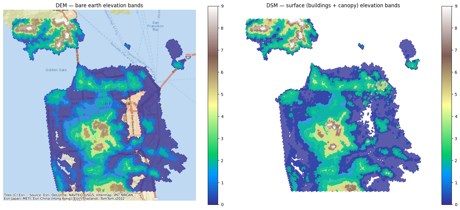
First, the surface stack over all of San Francisco — bare earth (DEM) beside the full surface (DSM), so buildings and canopy read as the difference between them:

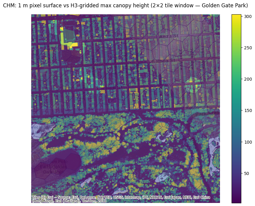
Zooming into one neighborhood, Part 3a cross-checks that the H3 grid faithfully summarizes the underlying 1 m pixels — a hex reads as the color of the pixels beneath it:

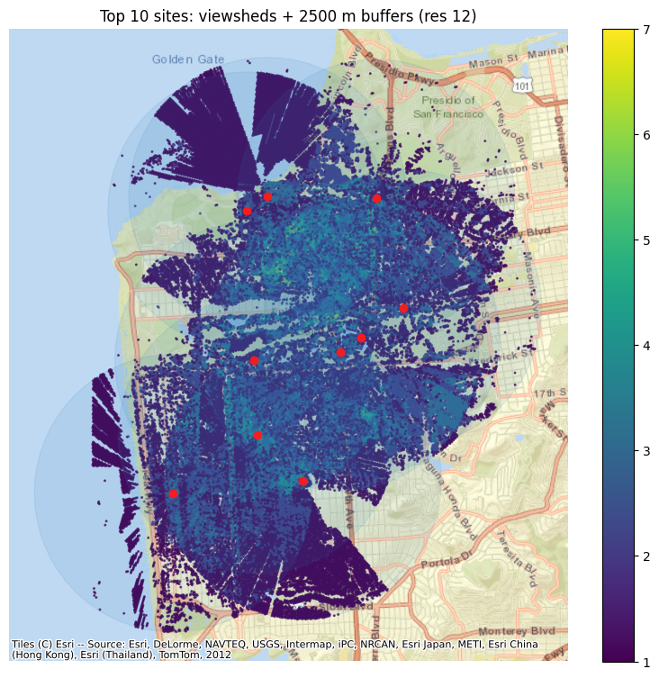
Finally — zooming to the Golden Gate Park demo, where the ranked sites are legible — Part 4 scores each candidate by how many res-12 cells it can see, so the best sites rise to the top:

---

Lakeflow SDP

A production-ready Wireless Coverage pipeline: a Lakeflow Declarative Pipeline (SDP) plus a post-pipeline tower-siting task, packaged as a Databricks Asset Bundle and running entirely on the GeoBrix lightweight tier over Serverless compute.

This is the production counterpart to the notebook series (see the other tab) — same San Francisco AOI and USGS 3DEP LiDAR sources, but running as a scheduled medallion pipeline instead of one-off notebook outputs: a land downloader task stages the data, then the pipeline cascades bronze → silver → gold through declared table-to-table dependencies, a siting task runs the H3-native tower analysis, and a validate notebook confirms all outputs.

View on GitHub

notebooks/examples/wireless-coverage/lakeflow — the bundle, pipeline transformations, siting task, validation notebook, and full setup instructions live here. See its README for deploy/run steps, prerequisites, and configuration notes.

Runs on the lightweight tier (Serverless)

The pipeline and its land and siting tasks install the GeoBrix wheel with the extra that matches the Lakeflow runtime — as of this example DBR 18.3, so geobrix[light_dbr18,vizx] (pipeline) and geobrix[light_env5,vizx] (serverless job tasks), both the protobuf-5 regime — as a single pip dependency entry; pure Python/PySpark bindings (databricks.labs.gbx.pyrx, pygx), no JAR, Serverless throughout. Lakeflow pins compute by a runtime channel: check the current Lakeflow runtime channel when you deploy and switch the extra to match if it has moved (e.g. DBR 19 → [light_dbr19]/[light_env6]). The bundle defaults to Serverless; for heavier runs (notably full San Francisco) you can switch the pipeline and job tasks to classic compute (serverless: false + a cluster spec) for dedicated memory and throughput. See Execution Tiers.

How it works: from staged LiDAR to ranked tower sites

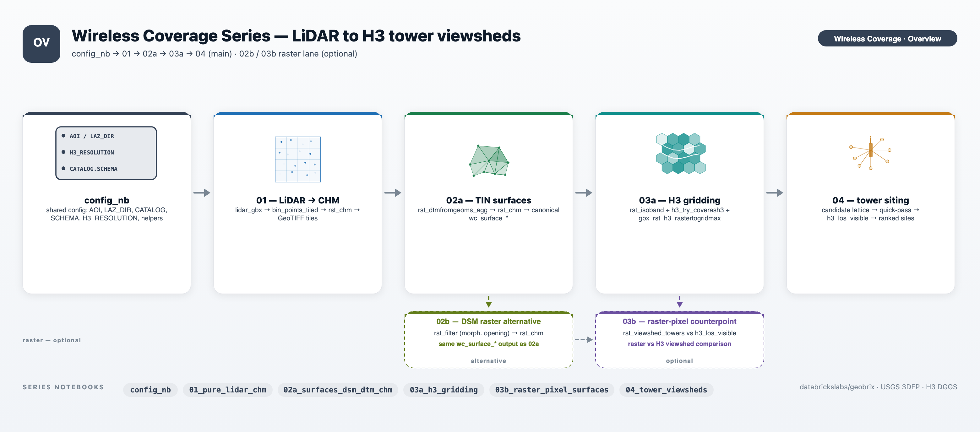
A scheduled run takes raw USGS 3DEP LiDAR .laz files through six stages:

1. Land — a downloader task stages USGS 3DEP LiDAR EPT nodes and Overture water polygons onto a Unity Catalog Volume. Nothing is interpreted yet — data just arrives.
2. Bronze — inventory — Auto Loader records one row per .laz file as it appears, so re-runs pick up only newly staged data.
3. Silver — surface stack — classified returns are tile-indexed and binned into 1 m DSM and TIN DTM rasters per tile; rst_chm derives the Canopy Height Model.
4. Gold — H3 grids — the surfaces are reprojected to EPSG:4326, isobanded, and indexed to H3 cells at resolution 10. Each table carries a stable res-9 join key so downstream consumers join on one column.
5. Siting — a post-pipeline Spark task runs the H3-native tower-siting analysis: a res-9 candidate lattice, a coarse quick-pass to rule out weak sites, and exact res-12 H3 line-of-sight viewsheds on survivors (distributed via h3_viewshed_towers — one tower per Spark task).
6. Validate — a final notebook task confirms all output tables are populated and spot-checks quality assertions.

Each stage reads only the one before it — declared as table-to-table dependencies — so Lakeflow builds the lineage graph, runs stages in order, and recomputes only what changed.

What a run looks like

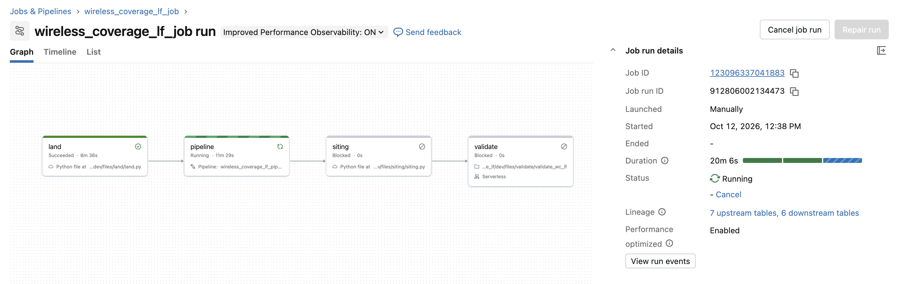
The bundle deploys one job, wireless_coverage_lf_job, whose four tasks run in sequence — land stages the data, pipeline refreshes the Lakeflow pipeline, siting ranks the tower sites, and validate checks the outputs:

Opening the pipeline task shows the medallion lineage Lakeflow derived from the table-to-table dependencies. On a full San Francisco run, ~817 M classified LiDAR returns (wc_lidar_pts) bin into a few hundred 1 m DSM / DTM / CHM surface tiles, which roll up into the res-10 H3 gold grids:

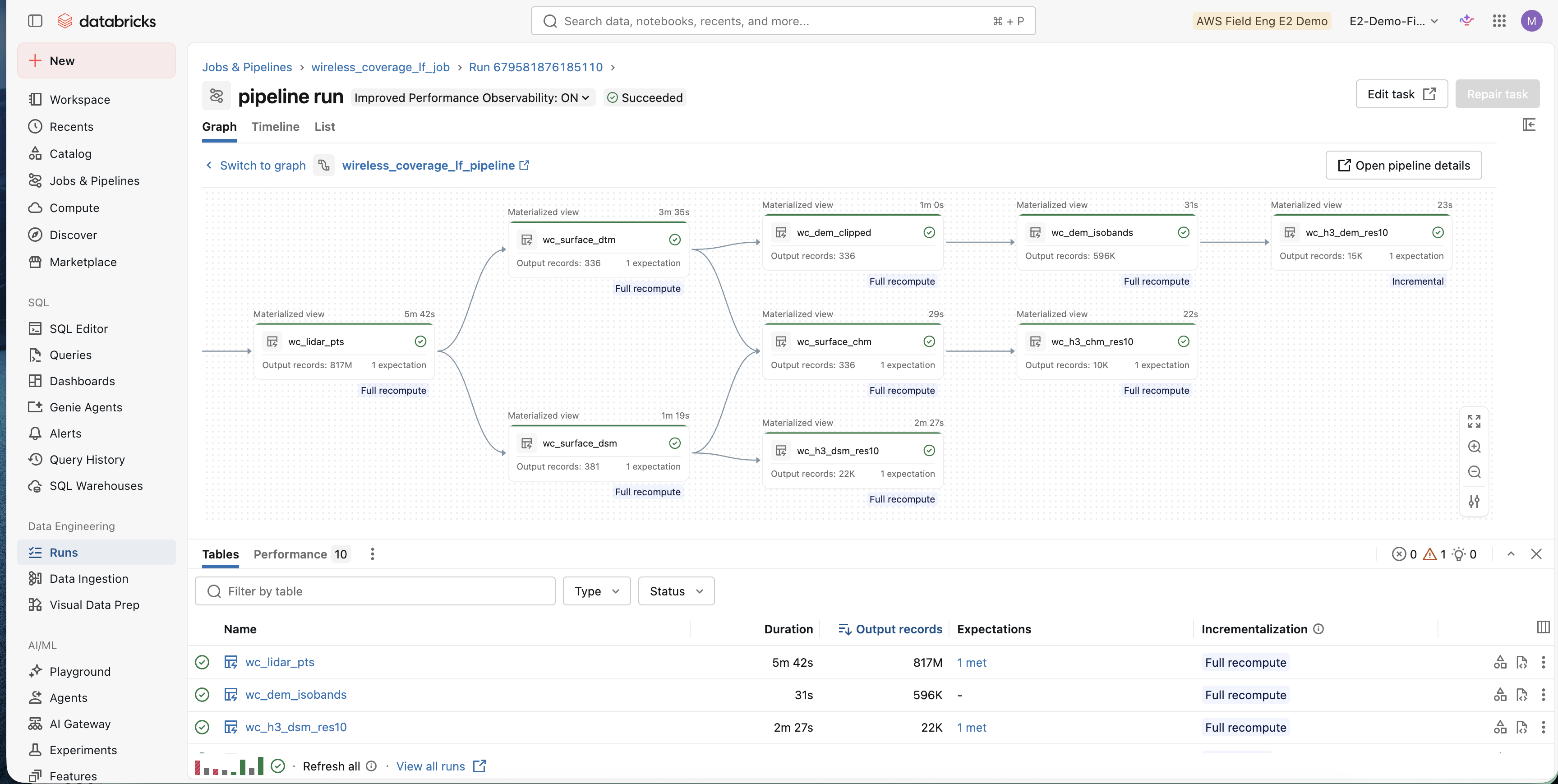
Table catalog

All tables land in {catalog}.{schema} (defaults: geospatial_docs.wireless_coverage_lf).

Bronze

Table	Description
laz_inventory	Auto Loader streaming table — one row per staged .laz EPT file (path, file_size, _ingested_at).

Silver

Table	Description
wc_lidar_pts	Classified LiDAR returns, tile-indexed with a res-15 H3 cell ID (EPSG:3857).
wc_surface_dsm	DSM — max elevation of all returns per 1 m tile.
wc_surface_dtm	DTM — Delaunay-TIN bare earth over class-2 ground returns (gap-free).
wc_surface_chm	CHM — rst_chm(DSM, DTM): canopy/structure height in metres, clamped ≥ 0.

Gold

Table	Description
wc_h3_dem_res10	Bare-earth elevation-band H3 cells (res 10), land-masked, with res-9 parent join key.
wc_h3_dsm_res10	Surface elevation-band H3 cells (res 10), land-masked, with res-9 parent join key.
wc_h3_chm_res10	Max canopy/structure height per H3 cell (res 10), gap-filled, land-masked, with res-9 parent join key.

Siting

The siting tables are regular Delta tables, overwritten each run. H3-indexed tables (*_res*) carry both a BIGINT cellid column and a STRING h3 column (for map tools that query string H3 keys) and are liquid-clustered on the BIGINT cell column for fast spatial queries. Coverage outputs are H3-indexed at resolution 12 and carry the res-9 parent join key.

Table	Description
wc_h3_surf_r13	H3 res-13 surface bin (DSM max elevation per cell) — finest-resolution blocker surface. Columns: cellid BIGINT, h3 STRING, z DOUBLE; liquid-clustered on cellid.
wc_h3_grnd_r13	H3 res-13 ground bin (DTM min elevation per cell) — finest-resolution bare-earth base. Columns: cellid BIGINT, h3 STRING, z DOUBLE; liquid-clustered on cellid.
wc_h3_quickpass_res9	Every res-9 candidate's coarse quick-pass coverage fraction (pre-rule-out screen).
wc_h3_candidate_sites_res9	Ranked tower survivors: cellid BIGINT, h3 STRING, lon, lat, required_mast, viewshed_cells, viewshed_pct, observer_z; liquid-clustered on cellid.
wc_h3_coverage_res12	Per-cell line-of-sight depth at res 12 — how many sited towers can see each cell. Columns: cellid BIGINT, h3 STRING, tower_los_count LONG, res INT, parent_cellid, parent_cellid_res; liquid-clustered on cellid. Suitable for external H3 map layers.
wc_h3_coverage_top10_res12	Same, aggregated over only the top-10 sites by coverage. Columns: cellid BIGINT, h3 STRING, tower_los_count LONG, res INT, parent_cellid, parent_cellid_res; liquid-clustered on cellid.
wc_h3_site_viewshed_res12	Per-site fine-resolution viewshed: one row per sited tower + visible cell pair. Columns: site_cellid BIGINT, site_h3 STRING, cellid BIGINT, h3 STRING, res INT, parent_cellid, parent_cellid_res; liquid-clustered on (site_cellid, cellid) for per-site lookups and per-cell map tiles.

Deploy and run

databricks bundle deploy
databricks bundle run wireless_coverage_lf_job

The bundle validates and deploys with the committed defaults in databricks.yml out of the box. To point it at your own workspace, copy databricks.override.yml.example to databricks.override.yml (git-ignored) and fill in your CLI profile; it is layered in automatically via include: ["*.override.yml"]. A fresh clone with no override file still validates/deploys.

• Schedule: the job ships paused (pause_status: PAUSED, daily at 0 0 7 * * ? America/Chicago) — unpause it in the workspace once you've confirmed a manual run.
• Shared LiDAR: if you have already run the notebook series and staged the USGS 3DEP data, set laz_dir (and optionally water_mask_dir) in your override file to reuse those files and skip the ~830 MB download. See databricks.override.yml.example for the exact paths.
• GeoBrix wheel: gbx_wheel points at a staged geobrix-0.5.2-py3-none-any.whl. Stage your own build at that path or override the variable to wherever your wheel lives.

Configuration

Catalog and schema names with hyphens

Unity Catalog catalog and schema names can include hyphens (e.g. solutions-catalog-default, sdsc-nyc-workshop-2026). Both the notebook series and the Lakeflow bundle properly quote all identifiers with backticks, so hyphenated names work without issue. If you encounter errors like "invalid identifier," check that your catalog/schema parameters are spelled correctly (case-sensitive).

Bundle variables (set in databricks.yml; override per-workspace in databricks.override.yml):

Variable	Default	Description
catalog	geospatial_docs	Unity Catalog catalog name.
schema	wireless_coverage_lf	UC schema; all pipeline and siting tables land here.
volume	data	UC volume; raw data lands under {volume}/wireless-coverage-lf/.
full_aoi	true	true for the full San Francisco AOI; false for the Golden Gate Park demo window.
simplify	true	Apply product st_simplify to isobands before H3 covering (default True = fast, no coverage loss, needed for full-SF performance; False = exact isobands, heavy/slow).
laz_dir	(derived)	Path to staged .laz EPT files. Leave empty to auto-derive under the Volume. Set to the notebook series' Volume path to reuse already-staged LiDAR.
water_mask_dir	(derived)	Path to staged Overture water GeoParquet. Leave empty to auto-derive.
gbx_wheel	/Volumes/geospatial_docs/geobrix/sample-data/geobrix-0.5.2-py3-none-any.whl	Path to the staged GeoBrix wheel.

Algorithm and resolution parameters are tunable via wireless_coverage.* keys in the pipeline configuration block. Key defaults:

Key	Default	Description
h3_res	10	H3 resolution for the gold elevation/canopy grids.
tower_res	9	H3 resolution for the naive candidate-tower lattice.
quickpass_res	10	Coarse quick-pass screen resolution.
viewshed_res	12	Exact H3 line-of-sight resolution (coverage output).
surface_bin_res	13	Finest H3 "pixel" bin resolution for siting surfaces.
max_dist_m	2500	Line-of-sight buffer radius in metres.
antenna_above_surface_m	10	Observer height above the DSM surface in metres.
quick_thresh_frac	0.30	Minimum quick-pass coverage fraction to survive rule-out.
simplify	true	Simplify isoband geometry via product st_simplify before H3 covering (default True; set False for exact isobands at the cost of heavy performance at full scale).

Prerequisites

• Unity Catalog: a catalog and schema (defaults geospatial_docs.wireless_coverage_lf) and a Volume named data under it. The pipeline creates sub-directories inside the Volume, not the Volume itself.
• GeoBrix wheel staged at the gbx_wheel path. See Execution Tiers.
• Network access: the land task fetches USGS 3DEP and Overture Maps data over HTTPS — Serverless has outbound internet by default.

Validation notebook

The validate task (validate/validate_wc_lf.ipynb) runs after the siting task completes, reads all output tables, confirms each is non-empty, and prints summary statistics. Run it manually from the workspace as a quick sanity check after a fresh deploy or configuration change.

Notebook Series

Wireless Coverage — LiDAR Surface Foundations

A notebook series that builds the elevation and surface data foundation for wireless-coverage analysis directly from a USGS 3DEP LiDAR point cloud — data first, analytics later. The surfaces produced here (Canopy Height Model, Digital Surface Model, bare-earth Digital Terrain Model) are the inputs that later parts consume for antenna siting via H3-native line-of-sight analysis.

The LiDAR path (Parts 1 and 2a) works over all of San Francisco (SF_AOI = (-122.55, 37.70, -122.35, 37.85)), reading the staged 3DEP LiDAR (.laz Entwine Point Tile nodes) with the GeoBrix lidar_gbx reader and binning returns into 1 m rasters per spatial tile. A single 1 m raster over SF is ~460 M pixels, so binning is tiled and bounded — rx.bin_points_tiled bins each tile with memory proportional to the raster grid (W×H), not the point count, so a full-resolution (DECIMATE=1) tile never OOMs. The binned surfaces are persisted to permanent tables you own (a CATALOG.SCHEMA you set) and read back downstream.

View on GitHub

notebooks/examples/wireless-coverage — download the folder and import the notebooks (Parts 1, 2a, 2b, 3a, 3b, and 4) into your Databricks workspace to run.

Runs on the lightweight tier (Serverless) by default

The series uses the lightweight tier — pure Python/PySpark bindings (databricks.labs.gbx.pyrx) plus the geobrix[light_env6,vizx] wheel — so it runs on Serverless environment 6 with no JAR or GDAL init script. The laspy / lazrs readers the point cloud needs ship with the light base. Visualization helpers come from databricks.labs.gbx.vizx. See Execution Tiers.

Big-data by default

DECIMATE=1 keeps every LiDAR return (~830 M over San Francisco) — an honest big-data run. Raise DECIMATE (e.g. 10) for a fast coarse pass while iterating on the visualization cells; the pipeline is identical either way.

The notebooks

Part 1 — Pure LiDAR → CHM (01_pure_lidar_chm.ipynb)

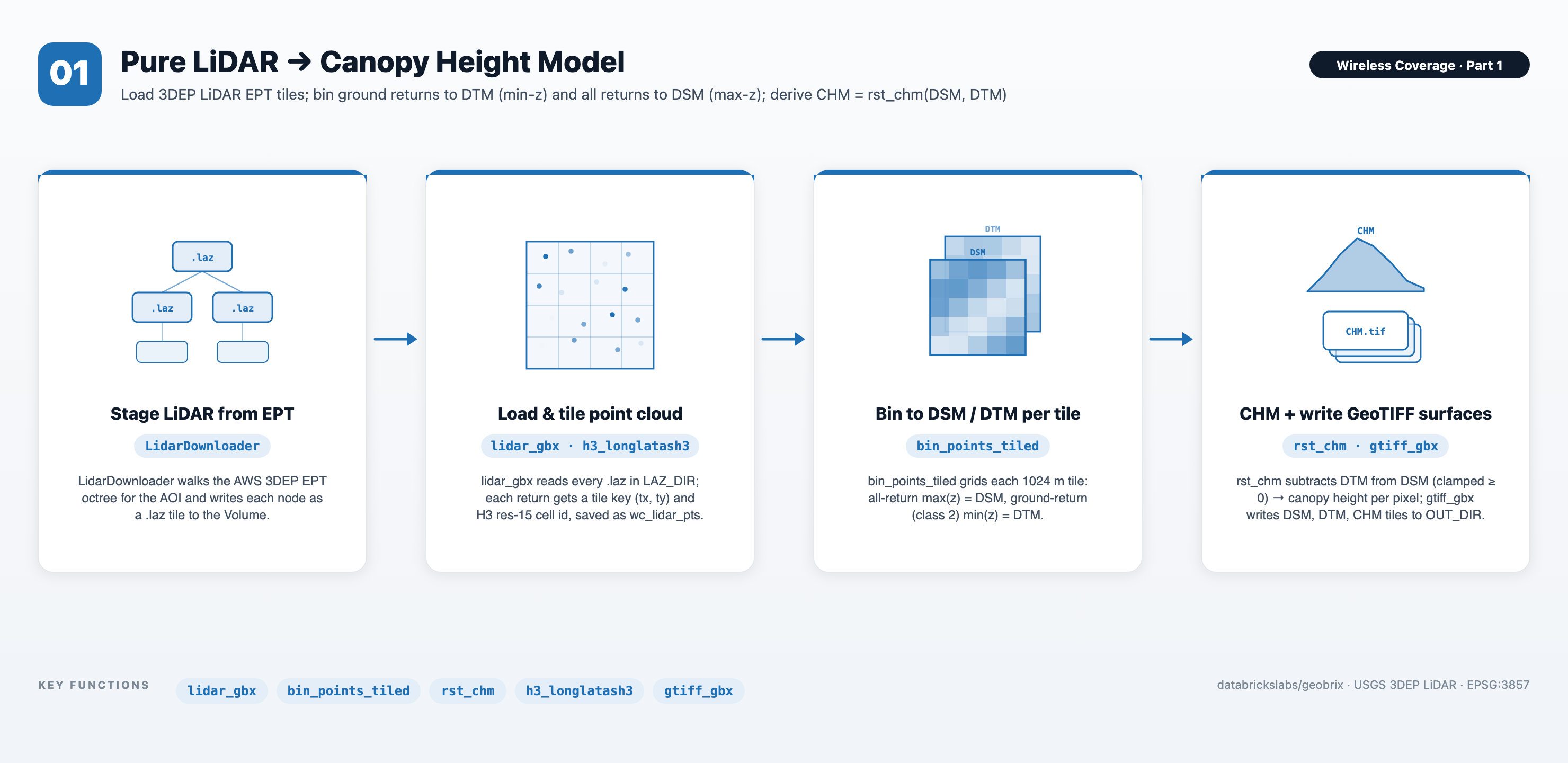
A classified LiDAR point cloud already carries everything a Canopy Height Model needs: every return is classified (ground vs. above-ground) and georeferenced. So the CHM is a couple of binning ops away — no external DEM, no coverage gaps:

• DTM (bare earth) — bin the ground returns (ASPRS class 2) → min elevation per pixel.
• DSM (surface) — bin all returns → max elevation per pixel.
• CHM — rst_chm(DSM, DTM) = DSM − DTM, clamped ≥ 0.

Part 1 is the shortest path from returns to canopy: it keeps only the CHM.

Part 2a — Surfaces: DSM + DTM → CHM (02a_surfaces_dsm_dtm_chm.ipynb)

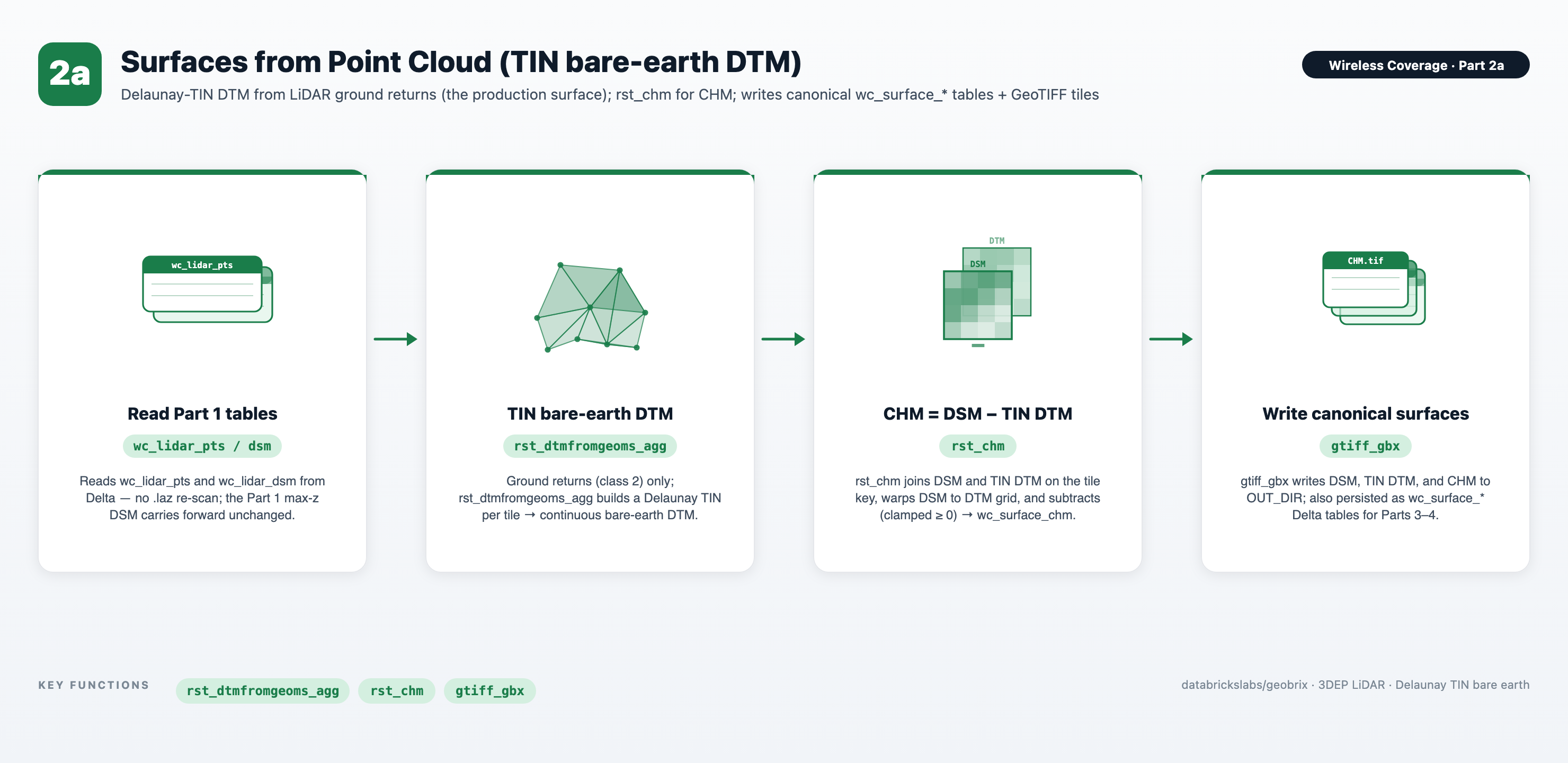
The main arc. Builds directly on the LiDAR point cloud from Part 1 and persists the complete surface stack as reusable permanent tables you own (a governed Delta table of tiles in a CATALOG.SCHEMA you set; optional GeoTIFF export via gtiff_gbx). The production bare-earth DTM is a TIN surface — a Delaunay triangulation of the classified ground returns (rst_dtmfromgeoms_agg), barycentrically interpolated to a gap-free raster. Because it works directly from the point cloud's own classification, it is a beyond-pixels surface: terrain reconstructed from the actual ground returns rather than approximated from raster values. The binned-min DTM is shown alongside for comparison:

• TIN DTM — a Delaunay triangulation of the ground returns (rst_dtmfromgeoms_agg), barycentrically interpolated to a gap-free bare earth. Points are built with st_makepoint(x, y, z), so Z carries through the WKB into the triangulation. This is the production terrain.
• Binned DTM — min z of ground returns per pixel (fast; can leave tiny gaps where no ground return landed). Shown for comparison.

Writes the canonical wc_surface_{dsm,dtm,chm} tables and OUT_DIR GeoTIFFs that Parts 3a, 3b, and 4 consume.

Part 2b — Surfaces from a DSM Raster (02b_surfaces_from_dsm.ipynb)

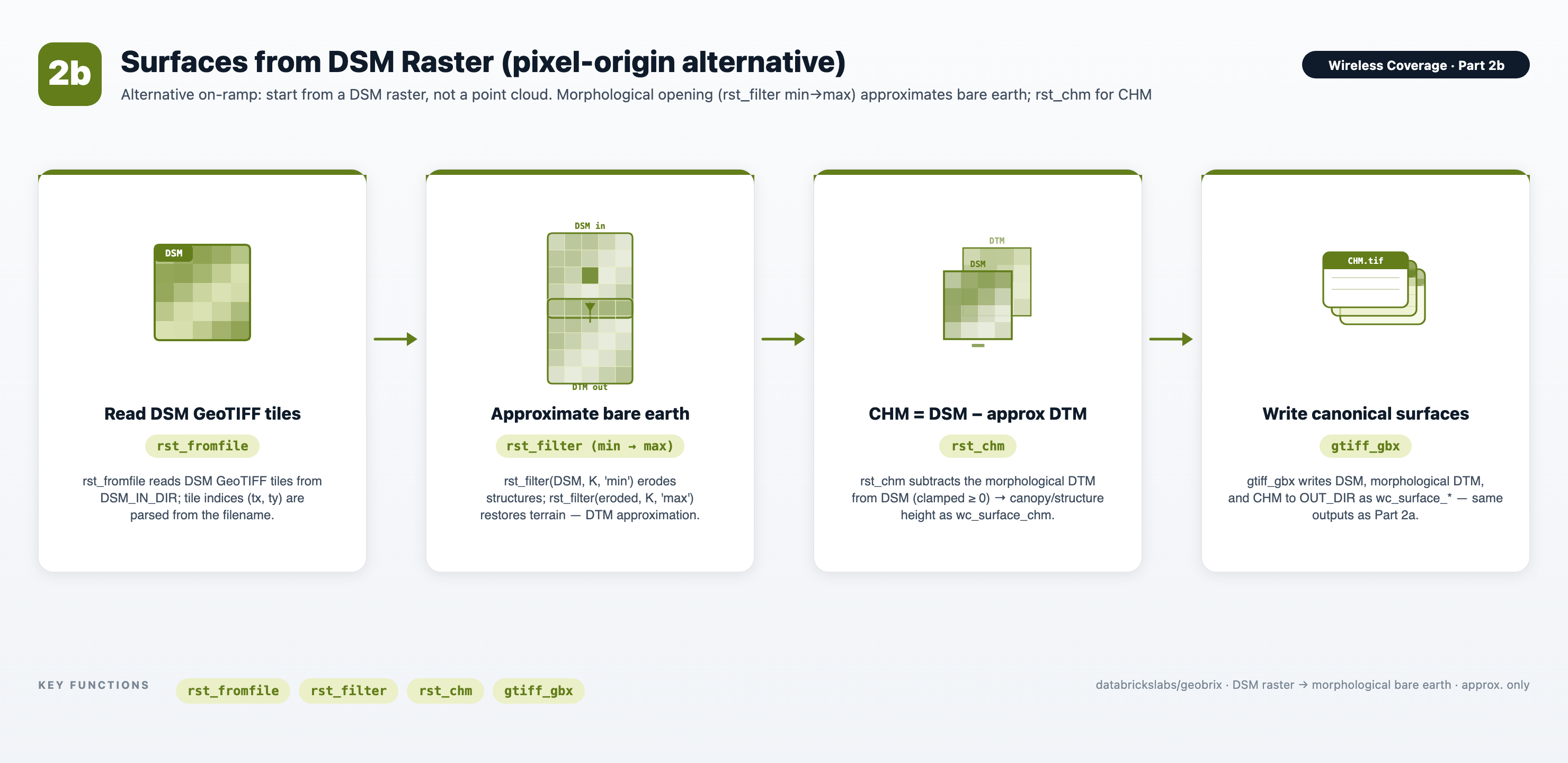
An alternative on-ramp for when a LiDAR point cloud is not available. Starting from a DSM raster only, it approximates the bare-earth DTM by applying a morphological opening to the DSM — rst_filter min then max — and then deriving the CHM with rst_chm. The result is a pixel-only approximation: without ground-classified returns, the bare earth is estimated from the surface shape rather than reconstructed from the point cloud. The Parts 1–2a LiDAR path produces a more accurate terrain for production use; when no point cloud is available, a published terrain product such as USGS 3DEP is the recommended production alternative. Part 2b lands the same canonical wc_surface_{dsm,dtm,chm} tables as Part 2a, so Parts 3 and 4 work unchanged either way.

Part 3a — H3 Gridding (03a_h3_gridding.ipynb)

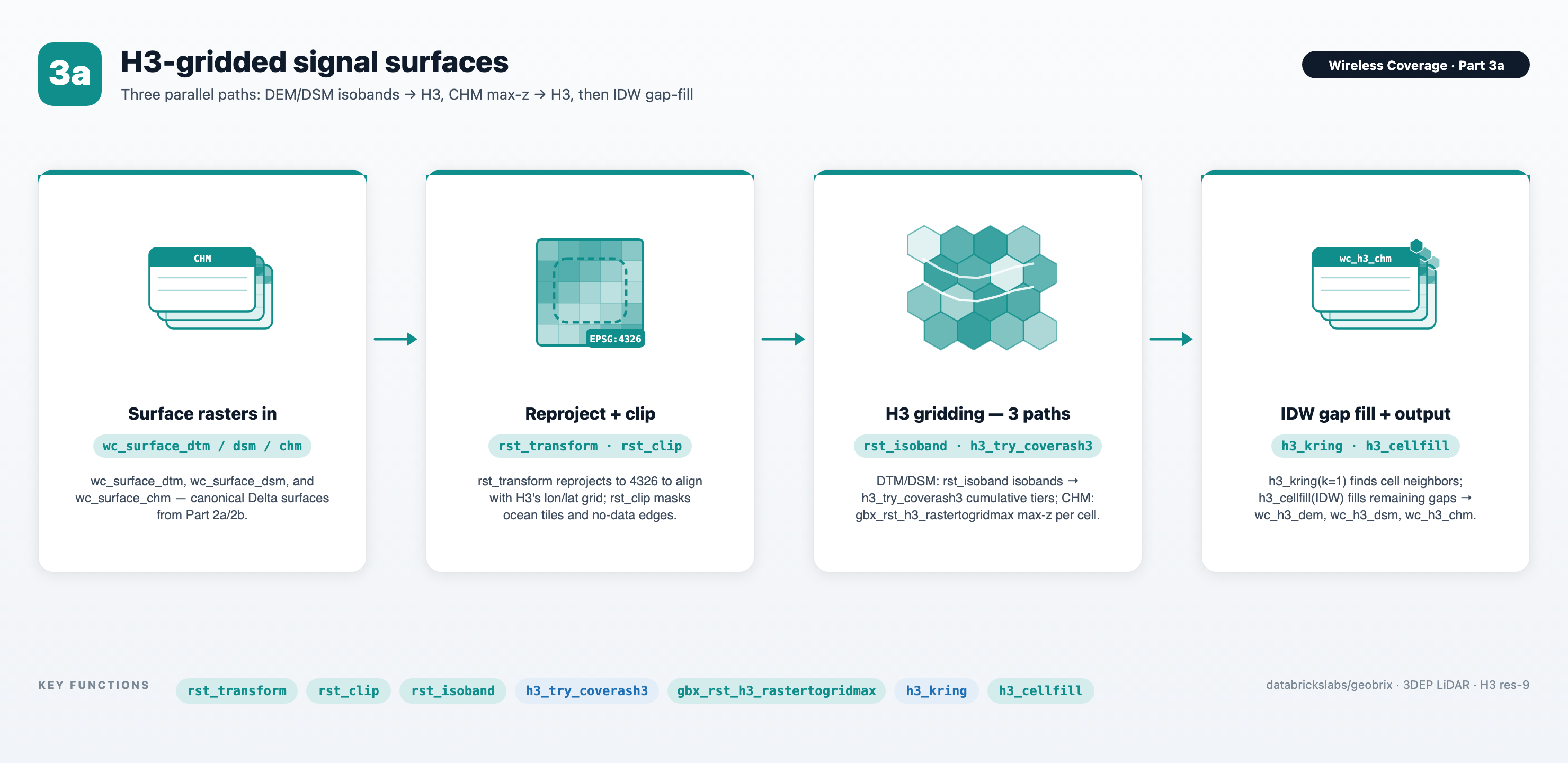
Takes the surface tables from Parts 1–2a (or 2b) and prepares them for global-grid analysis by H3-indexing each surface at a parameterized resolution (default: H3 resolution 10, ≈65 m edge). DEM and DSM elevation bands are extracted as contiguous isoband polygons via rst_isoband and indexed to H3 cells with the Databricks product h3_try_coverash3; cumulative elevation tiers give each cell a coverage-depth value. The Canopy Height Model is aggregated to the maximum canopy height per H3 cell via gbx_rst_h3_rastertogridmax. Interior gaps are filled with h3_cellfill (k=1, IDW, land mask re-applied after fill). All three H3 tables — wc_h3_dem, wc_h3_dsm, wc_h3_chm — are prepared for downstream analysis in Part 4. Each H3-cell output table carries a stable res-9 rollup join key — parent_cellid (the h3_toparent of each cell at res 9) and parent_cellid_res — so they join in one column to any external grid keyed at H3 resolution 9 (coverage, demand, population). This key is present on the Part 3a wc_h3_* tables, Part 4's wc_h3_coverage* tables, and Part 3b's wc_rpx_h3_coverage table.

H3 resolution is a choice, not a ceiling. Part 1 stored one res-15 cell per LiDAR return (cellid_r15, ≈0.9 m² — sub-metre, finer than a 1 m pixel). h3_toparent rolls any res-15 cell to any coarser resolution in a GROUP BY, so the same underlying data feeds res-10 visualization grids and res-12 viewshed buffers alike.

Part 3b — Raster-Pixel Surfaces (03b_raster_pixel_surfaces.ipynb)

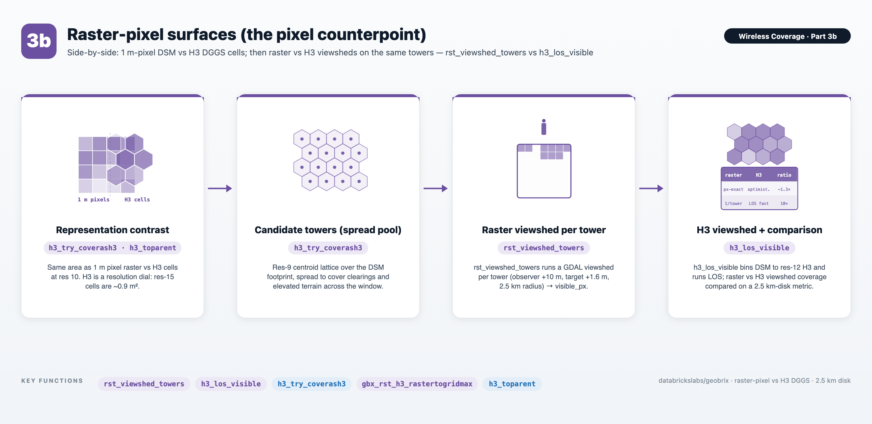
The honest counterpoint to Part 3a. Where Part 3a takes the LiDAR surfaces beyond pixels into an H3 discrete global grid, Part 3b holds the native 1 m raster representation up next to that H3 grid — and then re-runs Part 4's tower-siting question on the raster side so you can see how the two paradigms score the same ground.

Part A — representation contrast. Over a 2 km window around Golden Gate Park, the same DSM surface is rendered as 1 m-pixel tiles and as H3 cells at resolution 10. The contrast makes the resolution-dial framing concrete: the raster is fixed at 1 m; H3 dials to any resolution via h3_toparent. The res-15 cells stored in Part 1 (≈0.9 m² per cell — finer than a 1 m pixel) roll to resolution 10, 12, or any other target with a GROUP BY, so H3's resolution is a dial, not a ceiling.

Part B — viewshed foil. An independent spread of candidate towers over the DSM footprint is scored with the per-tower raster viewshed (rst_viewshed_towers) and, inline, the same res-12 H3 line-of-sight model (h3_los_visible) — so Part 3b runs standalone and the two engines are compared head-to-head. The candidate lattice regenerates Part 4's res-9 centroid pattern independently — Part 3b reads only the Part 2 DSM, Part 3a's H3 grids, and config_nb; it never touches a Part 4 table. rst_viewshed_towers selects the in-radius 1 m DSM tiles for each tower, mints a bytes-free VRT, runs one pixel-level viewshed, and histograms in-radius coverage — one tower per Spark task, the natural fan-out unit at full San Francisco scale. No raster bytes cross a shuffle.

The trade-off is stated honestly: Part 4's H3 viewshed bins one max-height per ~17 m res-12 cell, which smooths fine blockers that a 1 m raster line-of-sight respects. That makes the H3 viewshed an optimistic screening estimate — suitable for ruling out candidates quickly across the full lattice — while the raster viewshed is the strict pixel-level confirmation of a shortlisted site's exact coverage footprint. The large coverage gap between the two outputs is the expected signature of that resolution smoothing, not a defect in either approach.

Outputs (gated on FORCE_RELOAD; saved under the wc_rpx_ prefix):

Table	Contents
wc_rpx_raster_viewshed_demo	Per-tower raster coverage counts (visible_px, total_px, viewshed geometry)
wc_rpx_h3_viewshed_demo	Per-tower H3 line-of-sight cell counts (the H3-engine viewshed)
wc_rpx_h3_coverage_demo	Per-cell H3 LOS coverage depth for the demo towers
wc_rpx_comparison_demo	Raster vs H3 coverage area on the shared 2.5 km-disk metric

Maps — the strongest demo tower's exact 1 m-pixel viewshed next to Part 4's H3-cell coverage depth: two paradigms, one scene.

Part 4 — Naive H3-Native Tower Siting (04_tower_viewsheds.ipynb)

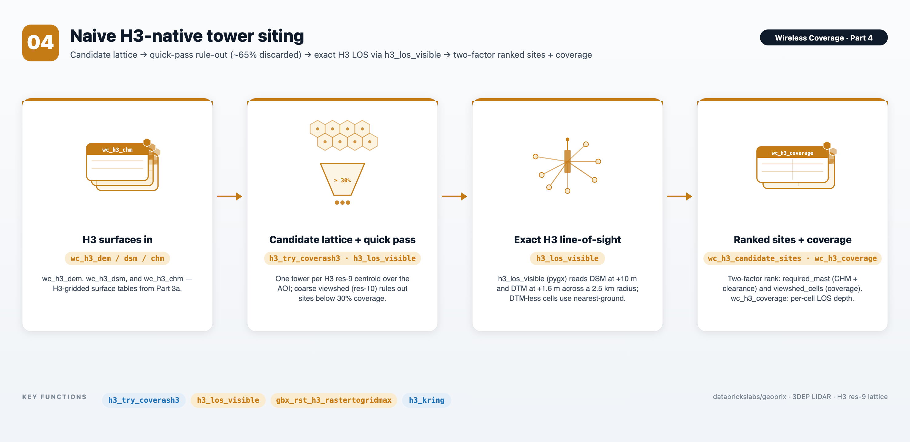
With the LiDAR surfaces from Parts 2a/2b and the H3 grids from Part 3a in hand, Part 4 asks the siting question: which candidate tower locations are worth the detailed analysis? The approach is deliberately naive — a baseline screen, not a final plan — and stays entirely in the H3 domain rather than operating on pixels.

Candidate lattice. One tower candidate is placed at the centroid of every H3 resolution-9 cell (≈170 m edge) that falls within the area of interest. No land-cover constraints, no placement optimization — just a dense, regular lattice that covers the whole AOI.

Quick-pass rule-out. Before paying for any detailed line-of-sight work, each candidate gets a cheap coarse viewshed at H3 resolution 10 (≈65 m). A site that cannot achieve at least 30% coverage of its buffer at that coarse resolution is ruled out immediately. In the Golden Gate Park demo, this reduces 176 candidates to 62 survivors (~65% discarded) before any fine-resolution work begins.

Exact H3 line-of-sight. Each surviving candidate is evaluated with the library function h3_los_visible (from databricks.labs.gbx.pygx) — a pure-Python H3 primitive that runs an exact ray-march test for every cell in the buffer. The observer sits at the DSM surface height plus a 10 m antenna clearance; the target is the ground surface (DTM) plus a 1.6 m receiver height. The buffer radius is 2.5 km. The line-of-sight test uses the binned H3 surface as both the blocker map and the ground reference, so it is a surface-relative check — the only shortcut is the H3 binning resolution, not the line-of-sight geometry.

Two-factor scoring. Each site is scored on two independent factors kept as separate columns:

• required_mast — the mast height the site needs to clear its own local surface and provide the 10 m antenna clearance (CHM + antenna_clearance; lower is cheaper to build).
• viewshed_cells — the number of H3 cells the site has line of sight to (higher is better coverage).

Sites are ranked by viewshed_cells descending, then required_mast ascending (nulls last). Combining the two into a single score — balancing cost against coverage — is a decision left to the analyst.

Nearest-ground fallback. Where a cell has a DSM surface value but no bare-earth DTM value (typical at water bodies or dense-canopy edges), the ground height for required_mast is filled from the mean of the nearest populated H3 ring (expanding up to 3 rings). A site with no ground anywhere in those rings keeps required_mast as NULL — honestly uncostable rather than guessed.

Outputs (all gated on FORCE_RELOAD; once the tables exist a re-run loads them and skips the per-tower viewsheds):

Table	Contents
wc_h3_quickpass	Every candidate's coarse coverage fraction (pre-rule-out score)
wc_h3_candidate_sites	Ranked survivors: required_mast, viewshed_cells, viewshed_pct, observer_z
wc_h3_coverage	Per-cell LOS depth: how many sited towers can see each H3 cell
wc_h3_coverage_top10	Same, aggregated over only the top-10 sites by coverage

Four maps trace the rule-out funnel: (A) all candidates colored by coarse coverage fraction; (B) survivors that cleared the quick-pass; (C) per-cell coverage depth with all sited towers and their 2.5 km buffers overlaid; (D) the ten best sites with their viewsheds and buffers.

Next. A forthcoming land_cover notebook adds the demand side — weighting coverage by where people and buildings are, excluding water, parks, and no-build zones — and optimizes placement within each cell, turning this naive screen into a smarter siting tool.

---

Table catalog

All notebook-series tables land in {CATALOG}.{SCHEMA} (defaults: geospatial_docs.geobrix). A demo run (DEMO=True) appends a _demo suffix so it never collides with a full-SF run; H3 tables append _res{n}.

The series shares most of its outputs with the Lakeflow SDP flavor — the same table names, but written to a different schema (geospatial_docs.wireless_coverage_lf). The last column contrasts the two flavors.

Table	From	Description	Lakeflow (LDP) flavor
wc_lidar_pts	01	Classified LiDAR returns, tile-indexed with a res-15 H3 cell ID (EPSG:3857).	Shared (LDP Silver)
wc_lidar_dsm / wc_lidar_dtm / wc_lidar_chm	01	Part 1's shortest-path DSM / bin-min DTM / CHM surfaces, kept for the pure-LiDAR walkthrough.	Notebook-only (LDP builds wc_surface_* instead)
wc_surface_dsm	02a / 02b	DSM — max elevation of all returns per 1 m tile.	Shared (LDP Silver)
wc_surface_dtm	02a / 02b	DTM — Delaunay-TIN bare earth (02a) or morphological-opening approximation (02b).	Shared (LDP Silver; the LDP uses the TIN path)
wc_surface_chm	02a / 02b	CHM — rst_chm(DSM, DTM), clamped ≥ 0.	Shared (LDP Silver)
wc_h3_dem_res10 / wc_h3_dsm_res10 / wc_h3_chm_res10	03a	Land-masked elevation-band DEM/DSM and the raw max-canopy (CHM) grid — H3 cells at res 10 with a res-9 parent join key. nb3a clamps, gap-fills, and land-masks the CHM in-notebook for the rendered/analysis surface.	Shared (LDP Gold)
wc_rpx_raster_viewshed / wc_rpx_h3_viewshed / wc_rpx_h3_coverage / wc_rpx_comparison	03b	Raster-pixel vs H3 viewshed comparison — 1 m-pixel rst_viewshed_towers vs res-12 h3_los_visible, head-to-head on the same towers.	Notebook-only (no raster-pixel stage in the LDP)
wc_h3_surf_r13 / wc_h3_grnd_r13	04	Res-13 surface (DSM max) and ground (DTM min) bins — the finest blocker/base for line-of-sight.	Shared (LDP Siting)
wc_h3_quickpass_res9	04	Every res-9 candidate's coarse quick-pass coverage fraction (pre-rule-out screen).	Shared (LDP Siting)
wc_h3_candidate_sites_res9	04	Ranked tower survivors: cellid BIGINT, h3 STRING, lon, lat, required_mast, viewshed_cells, viewshed_pct, observer_z (liquid-clustered on cellid).	Shared (LDP Siting)
wc_h3_coverage_res12 / wc_h3_coverage_top10_res12	04	Per-cell line-of-sight depth at res 12 (all sites / top-10), H3-indexed with cellid BIGINT, h3 STRING columns (liquid-clustered on cellid), and the res-9 parent join key.	Shared (LDP Siting)
wc_h3_site_viewshed_res12	04	Per-site fine-resolution viewshed: one row per sited tower + visible cell pair. Columns: site_cellid BIGINT, site_h3 STRING, cellid BIGINT, h3 STRING (liquid-clustered on (site_cellid, cellid) for per-site lookups and per-cell map tiles).	Shared (LDP Siting)
laz_inventory	—	(not generated by the notebook series)	Lakeflow-only — a Bronze Auto Loader stream; the notebooks read the staged .laz directly via lidar_gbx.

Key GeoBrix functions shown

• lidar_gbx reader — spark.read.format("lidar_gbx").option("decimate", …).load(path) emits one Spark row per LiDAR return (x, y, z, intensity, return_number, number_of_returns, classification, gps_time), recursing sub-directories of staged .laz. Options: classFilter, returnFilter, decimate, mode (points / metadata). See LiDAR reader.
• bin_points_tiled — bounded tiled point binning: peak memory is the raster grid (W×H), not the point count, so full-density LiDAR bins without OOM. Picks a per-pixel statistic (max for the DSM surface, min on ground returns for the bare-earth DTM) and is built on rst_binpoints_agg. See RasterX › Memory & scale.
• rst_chm — differences an aligned DSM and DTM into a Canopy Height Model (DSM − DTM, clamped ≥ 0, NoData preserved). See RasterX functions.
• rst_dtmfromgeoms_agg — builds a Delaunay-TIN bare-earth surface from ground points (and optional breaklines) with barycentric interpolation — a gap-free alternative to the binned min DTM. Points arrive as WKB POINT Z from the product st_makepoint(x, y, z). See RasterX functions.
• gtiff_gbx writer — df.select("source", "tile").write.format("gtiff_gbx").mode("overwrite").save(dir) writes each raster tile as a GeoTIFF (<source>.tif) to a Volume. See GeoTIFF writer.
• gbx.vizx helpers — plot_raster / plot_file render tiles and staged GeoTIFFs (auto-decimation + percentile stretch, cmap=). See Visualization API.

---

Data flow

Staged 3DEP LiDAR (.laz EPT nodes)  →  lidar_gbx reader  →  one row per return (x, y, z, classification, …; EPSG:3857)
        │
        ▼  assign tile keys (tx, ty) + per-tile extent columns (1024 m tiles, 1 m pixels)
        │
        ├─▼  bin_points_tiled(all returns, "max")  per tile (bounded)  →  DSM tiles
        └─▼  bin_points_tiled(class 2,      "min")  per tile (bounded)  →  DTM tiles (bare earth)
        │
        ▼  rst_chm(DSM, DTM)  (Spark, per tile)
Canopy Height Model tiles  (Float32, NoData = −9999)
        │
        ▼  (Part 2a) _persist  →  DSM / DTM / CHM permanent tables (CATALOG.SCHEMA); optional gtiff_gbx GeoTIFF export
        ▼  (Part 2a) rst_dtmfromgeoms_agg on st_makepoint(x, y, z) ground points  →  TIN bare earth (gap-free)
        ▼  (Part 2b, alt) DSM raster in  →  rst_filter(min→max) morphological open  →  approximate bare earth; rst_chm  →  same surface tables (pixel-only path)
        │
        ▼  (Part 3a) rst_isoband → h3_try_coverash3  →  wc_h3_dem / wc_h3_dsm elevation-tier grids
        ▼  (Part 3a) gbx_rst_h3_rastertogridmax  →  wc_h3_chm max-canopy grid
        ▼  (Part 3a) h3_cellfill (k=1, IDW, land mask)  →  gap-filled H3 tables
        │
        ▼  (Part 3b) independent candidate lattice  →  rst_viewshed_towers (per-tower, 1 m raster)  →  wc_rpx_raster_viewshed_demo
        ▼  (Part 3b) h3_los_visible (inline, res-12, self-contained)  →  wc_rpx_h3_viewshed_demo / wc_rpx_h3_coverage_demo
        ▼  (Part 3b) raster vs H3 comparison  →  wc_rpx_comparison_demo
        │
        ▼  (Part 4) H3 res-9 centroid lattice  →  quick-pass rule-out (res-10, 30% threshold)
        ▼  (Part 4) h3_los_visible (res-12, 2.5 km buffer)  →  wc_h3_candidate_sites
        ▼  (Part 4) per-cell LOS depth aggregation  →  wc_h3_coverage / wc_h3_coverage_top10

---

Gotchas

• Bin per tile, bounded. A single 1 m raster over all of San Francisco is ~460 M pixels — far too large for one tile. rx.bin_points_tiled assigns per-tile extents and bins each tile with memory bounded by the grid (W×H), not the point count, so full-density (DECIMATE=1) binning never OOMs. (Calling rst_binpoints_agg directly realizes a whole tile's points and can exhaust RAM at full density — see Memory & scale.)
• Ground is ASPRS class 2. The bare-earth DTM bins only classification 2 (ground); the DSM bins all returns. Filtering the point DataFrame to class 2 before the min bin is what makes the DTM "bare earth."
• Z must survive to the TIN. rst_dtmfromgeoms_agg needs POINT Z geometry. Build points with the product st_makepoint(x, y, z) and pass st_asbinary(...) — the WKB carries Z, so the triangulation interpolates real elevations rather than collapsing to 2D.
• Thin the points that feed the TIN. A Delaunay TIN holds all its points in memory to triangulate — unlike the binned DTM (memory bounded by the raster grid), a triangulation is inherently global and can't be grid-bounded. At DECIMATE=1 a single tile's ground returns can exhaust a worker, so Part 2a samples them to a bounded count (TIN_MAX_PTS) before triangulating; a bare-earth TIN is near-identical from a representative subset. See RasterX › Memory & scale.
• Empty / corrupt point-cloud nodes are skipped. The lidar_gbx reader skips 0-byte or unreadable .laz files with a warning instead of failing the whole distributed read, so one bad EPT node can't take down the job.
• Serverless-safe throughout. No spark.conf.set, _jvm, .rdd, .cache() / .persist(). Surfaces are persisted to permanent tables you own (CATALOG.SCHEMA) — a governed Delta table of tiles, reused across cells and sessions rather than a session temp table. An optional gtiff_gbx export writes GeoTIFF files to a Volume.

---

Related

• DEM extra — H3 Rasterize takes the complementary path: a ready-made 10 m seamless DEM over the Bay Area run through the full raster→H3 pipeline (rst_clip → rst_isoband → product H3 → rst_h3_rasterize_agg → rst_frombands_agg). No LiDAR required — it shows the "if the elevation raster already exists" route to the same kind of coverage-tier model.