H3 Rasterize — Polygon Isobands to Multi-Band H3 Raster Stack
An end-to-end example showing how to convert arbitrary polygon isobands — elevation contours, signal-strength coverage zones, or any threshold-derived footprint — into a pixel-aligned, multi-band H3 raster stack using GeoBrix RasterX and the lightweight gbx.vizx helpers.
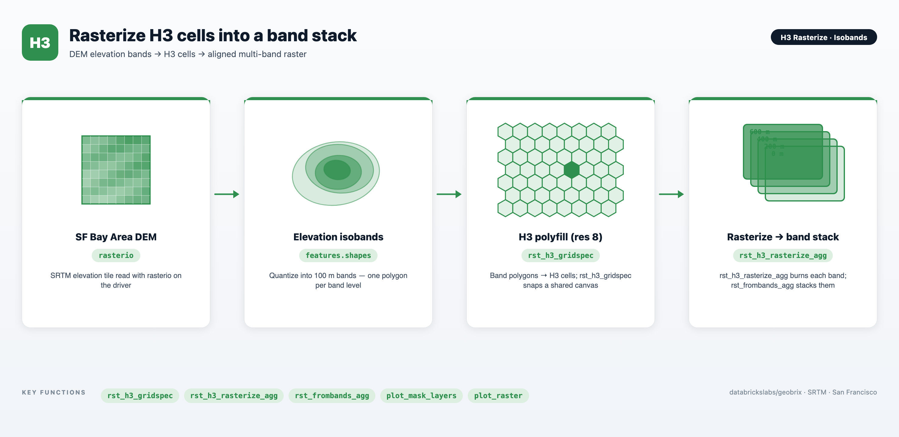
The notebook works through the San Francisco Bay Area: it reads a 1°×1° SRTM DEM tile (srtm_n37w123.tif, EPSG:4326) covering the SF Peninsula, Marin headlands, and East Bay hills, extracts eight 100 m elevation bands (0–700 m), polyfills each band with H3 resolution-8 hexagons, computes a shared pixel grid that spans all bands with rst_h3_gridspec, burns each band onto that grid with rst_h3_rasterize_agg, and assembles all eight single-band tiles into one multi-band GeoTIFF with rst_frombands_agg. A coverage-depth composite rendered by plot_raster closes the loop, showing at a glance how many elevation bands cover each pixel.
notebooks/examples/h3-rasterize — download h3_rasterize_isobands.ipynb and import it into your Databricks workspace to run.
geobrix[light,vizx])The notebook uses the lightweight tier — pure Python/PySpark bindings (databricks.labs.gbx.pyrx) plus the geobrix[light,vizx] wheel — so it runs on Serverless with no JAR or GDAL init script. The per-band rasterize result is materialized into a session-scoped temporary table (CREATE TEMP TABLE) so that the stacking step reads cached bytes instead of recomputing the burn. Session temp tables require Serverless or DBR 18.1+; they are not supported on dedicated / single-user clusters. See Execution Tiers for the trade-offs between lightweight and heavyweight.
Files
| File | Purpose |
|---|---|
h3_rasterize_isobands.ipynb | The full pipeline: DEM staging, isoband extraction, H3 polyfill, shared grid spec, per-band rasterize, band stacking, and visualization. |
README.md | Setup instructions, requirements, and a summary of each pipeline step. |
Prerequisites
- Databricks Runtime 17.3 LTS / 18.1+ or Serverless (Spark 4 / Python 3.12). Lightweight default runs on Serverless. Session temp tables (Step 4) require Serverless or DBR 18.1+; they are not available on dedicated / single-user clusters.
- GeoBrix (version 0.4.0). The
%pip installcell installs thegeobrix[light,vizx]wheel, which pulls inrasterio(used for the driver-side DEM read and isoband extraction),h3(polyfill),matplotlib,geopandas, andmapclassify(visualization). No JAR or GDAL init script is required. - Unity Catalog Volume: the DEM is staged to
/Volumes/geospatial_docs/geobrix/sample-data/geobrix-examples/sf/elevation/srtm_n37w123.tif. UpdateDEM_PATHif your Volume layout differs. The Volume root must already exist; the staging cell creates sub-directories but not the root. - Wheel path: update the
%pip installcell to point at your stagedgeobrix-0.4.2-py3-none-any.whlif its Volume path differs from the default.
Run order
- Install and restart — the
%pip installcell installsgeobrix[light,vizx]and is followed immediately by%restart_python; run cells in order without skipping the restart. - Imports and registration — imports
pyrx,gbx.vizxhelpers, and callsrx.register(spark)+register(spark)to install SQL UDFs. - Stage the DEM — the staging cell downloads
srtm_n37w123.tiffrom public AWS Terrain Tiles to the Volume (idempotent; skipped if the file already exists). - Steps 1–2 (driver) — DEM read, isoband extraction, and H3 polyfill all run on the driver via
rasterioandh3. A Spark DataFrame is created from the resulting(band_level, cellid)rows. - Steps 3–5 (Spark) —
rst_h3_gridspec(shared canvas),rst_h3_rasterize_agg(per-band burn → materialized temp table), andrst_frombands_agg(multi-band stack) fan out across executors.
Data flow
srtm_n37w123.tif  (SRTM, EPSG:4326, AWS Terrain Tiles → UC Volume)
        │
        ▼  rasterio + rasterio.features.shapes (driver)
Elevation isobands  (8 GeoJSON polygon groups, 0–700 m, 100 m step)
        │
        ▼  h3.polygon_to_cells @ resolution 8 (driver)
(band_level, cellid) DataFrame  (~12 000 rows after dedup)
        │
        ▼  rx.rst_h3_gridspec (Spark)
Shared grid spec  (xmin/ymin/xmax/ymax/width/height, single canvas for all bands)
        │
        ▼  rx.rst_h3_rasterize_agg grouped by band_level (Spark) → TEMP TABLE
Per-band presence tiles  (8 × 499×505 px, 1-band each, NoData = not covered)
        │
        ▼  rx.rst_frombands_agg ordered by band_level (Spark)
Multi-band GeoTIFF stack  (1 tile, 8 bands, 499×505 px, EPSG:4326)
        │
        ▼  plot_raster(composite="depth") + plot_mask_layers / cells_as_gdf / grid_as_gdf
Coverage-depth composite + per-band footprint overlays
Key GeoBrix / Databricks functions shown
rst_h3_gridspec— computes a pixel-snapped bounding box and pixel dimensions spanning all H3 cells across all band levels; used without a grouping column here to produce a single shared canvas. See H3 Grid.rst_h3_rasterize_agg— aggregator that burns a group's H3 cells onto the shared canvas (supplied explicitly viaxmin/ymin/xmax/ymax/width/heightcolumns), producing a single-band presence mask per band level. See H3 Grid.rst_frombands_agg— aggregator that assembles per-band single-band tiles into one multi-band GeoTIFF, ordered by a user-suppliedband_indexcolumn.gbx.vizxhelpers (Visualization API):plot_mask_layers— overlays two or more named binary masks on a single figure, each in a distinct colour with a legend, for side-by-side band coverage comparison.plot_raster(composite="depth")— renders the stacked tile as a coverage-depth heatmap: per-pixel count of bands that cover that location, transparent where no band covers.grid_as_gdf— converts thegridstruct fromrst_h3_gridspecinto a single-row GeoDataFrame for map overlays.cells_as_gdf— converts a(cellid, ...)DataFrame into a GeoDataFrame (one hexagon polygon per row) for matplotlib or interactive map visualization.
Gotchas
- Session temp table requires Serverless or DBR 18.1+: the notebook materializes per-band tiles with
CREATE OR REPLACE TEMP TABLE(via a temp view bridge) to avoid recomputing the burn in the stacking step. On Serverless.cache()/.persist()are unavailable; a session temp table is the idiomatic alternative. This syntax is not supported on dedicated or single-user clusters — if you must run there, remove the temp-table step and passbands_dfdirectly intorst_frombands_agg(at the cost of recomputing the rasterize). - Driver-side DEM steps are intentional: isoband extraction and H3 polyfill run on the driver because the notebook reads a single DEM tile. For a production pipeline that ingests many tiles, load the DEM files into a Spark DataFrame via
spark.read.format("binaryFile")or thegtiff_gbxreader (one row per file) and move both steps into a pandas UDF or UDTF so they fan out per tile across executors. - Shared canvas is required for stacking: all per-band tiles passed to
rst_frombands_aggmust have identical pixel dimensions (width × height) and spatial extent. Broadcasting thexmin/ymin/xmax/ymax/width/heightliterals fromrst_h3_gridspecto every row before grouping ensures this. Mismatched extents produce a corrupt or truncated stack. - Cell-ID encoding:
h3.polygon_to_cellsreturns string hex IDs; the notebook converts them to 64-bit integers viah3.str_to_intbecause PySpark mapsLongTypeto ScalaLong. Pass integer cell IDs torst_h3_rasterize_agg; string IDs will fail at runtime. - Coordinate ordering for
h3.LatLngPoly:rasterio.features.shapesreturns GeoJSON(lon, lat)tuples;h3.LatLngPolyexpects(lat, lon). The notebook swaps the pair explicitly in the polyfill loop — omitting this swap shifts the polyfill to the wrong hemisphere. - Volume write is sequential (FUSE-safe): the DEM staging cell copies the converted GeoTIFF to the Volume via
shutil.copyfrom a node-local temp directory. This is the correct pattern for Unity Catalog Volume writes on Serverless: avoidseek, use sequential I/O, and never write directly into/tmppaths that are not node-local scratch.