Clipping - xView — Per-Object Raster Clipping with GeoBrix
An end-to-end example showing how to load high-resolution aerial GeoTIFFs from the xView Detection Challenge dataset into Lakehouse tables and clip rasters to labeled objects in the accompanying GeoJSON, using GeoBrix RasterX together with Databricks built-in Spatial SQL functions.
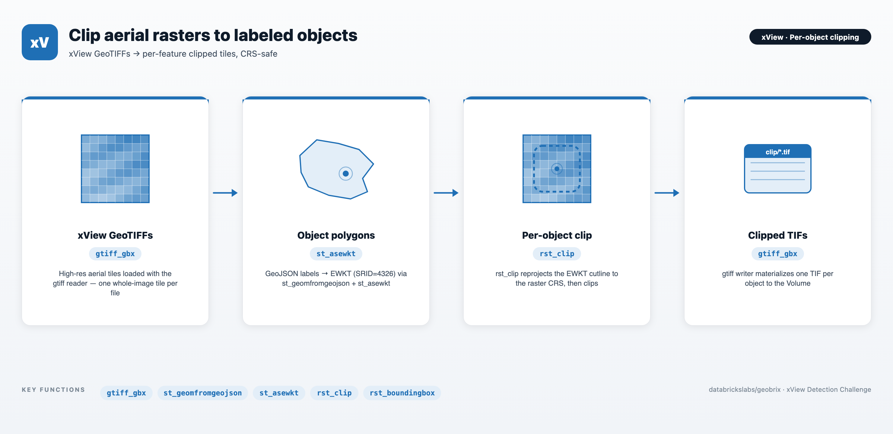
The single notebook moves from raw xView TGZ archives → a raster table loaded by the built-in gtiff reader → GeoJSON-derived object table (EWKT with SRID) → per-object clipped tiles, written back to a Unity Catalog Volume as individual TIFs by the built-in gtiff writer.
notebooks/examples/xview — download Clipping - xView.ipynb and import it into your Databricks workspace to run.
The notebook uses the lightweight tier — pure Python/PySpark bindings (databricks.labs.gbx.pyrx) plus the geobrix[light] wheel — so it runs on Serverless with no JAR. To run it on the heavyweight tier instead, make a few tweaks: swap the import to databricks.labs.gbx.rasterx (the commented option-2 in the setup cell) and, on a classic x86 cluster, attach both the GeoBrix JAR and the GDAL init script that installs the native GDAL libraries the JNI bindings load. Either way the in-notebook preview cells need rasterio — install it directly (%pip install rasterio) or pull it in via the geobrix[light] extra. See Execution Tiers for the trade-offs.
You need a free account at challenge.xviewdataset.org to obtain session-based download links for xView_train.tgz (training imagery) and the labels archive. Paste those URLs into the train_url / labels_url cells before running the download step.
Files
| File | Purpose |
|---|---|
Clipping - xView.ipynb | The full pipeline. Sets up the catalog / schema / Volume, downloads + extracts the xView training TGZ and label GeoJSON to /Volumes/<cat>/<schema>/data/, loads rasters with the gtiff reader (one whole-image tile per .tif), builds an object table from xView_train.geojson via st_geomfromgeojson + st_asewkt, joins objects to their source tiles, applies rst_clip(tile, wkt_clip, True) with EWKT-encoded polygons, and writes the clipped rasters back to the Volume with the gtiff writer as <index_right>_<type_id>_<feature_id>.tif. |
Prerequisites
- Databricks Runtime 17.3 LTS / 18 LTS, or Serverless (Scala 2.13 / Spark 4 / Python 3.12). The lightweight default runs on Serverless; the heavyweight tweak needs a classic x86 cluster.
- GeoBrix (version 0.4.0). The setup cell
%pip-installs thegeobrix[light]wheel, which brings the pure-Python bindings (databricks.labs.gbx.pyrx) and their dependencies (includingrasterio, used for the in-notebook previews). For the heavyweight tweak, also attach the GeoBrix JAR and the GDAL init script to the cluster, and switch the import todatabricks.labs.gbx.rasterx. - Unity Catalog: set
catalog_name/schema_nameat the top of the notebook. A Volume nameddatamust already exist under<catalog>/<schema>; the notebook will create the schema but not the Volume. - Compute sizing: xView training tiles are ~3000×3000 RGB GeoTIFFs. For the heavyweight tier, an x86 cluster is required for the GDAL JNI natives, and memory/disk-optimized variants (e.g.
r6id.*,m5d.*) are recommended for the raster-processing step.
Pipeline
xView train TGZ + xView_train.geojson  (session-signed downloads)
          │
          ▼  download_extract → /Volumes/<cat>/<schema>/data/{train_images, train_labels}
gtiff reader over train_images/*.tif  (one whole-image tile per file)
          │
          ▼  + rst_boundingbox + rst_srid                 →  xview_raster
GeoJSON objects (features)
          │
          ▼  st_geomfromgeojson → st_asewkt (SRID=4326)   →  xview_object
Join objects to rasters on image_file (basename)
          │
          ▼  rst_clip(tile, wkt_clip, True)                →  xview_object_clip
gtiff writer (nameCol)
          │
          ▼  /Volumes/<cat>/<schema>/data/clip/<index_right>_<type_id>_<feature_id>.tif
Key GeoBrix / Databricks functions shown
- GeoBrix RasterX (
rx.rst_*):rst_boundingbox,rst_srid,rst_summary,rst_clip(with EWKT input). - Databricks built-in ST (
DBF.*):st_geomfromgeojson,st_asewkt— used to emit each feature's polygon asSRID=4326;POLYGON(...)so that the SRID travels with the WKT intorst_clip. - Readers: the GeoBrix
gtiffreader (format("gtiff_gbx")) loads each.tifstraight into atilecolumn — the defaultsizeInMB=-1means no windowed split, i.e. one whole-image tile per file, so every label clips against the single tile that contains it;json(multiline) reads the xView labels GeoJSON. Readers/writers are installed byregister(spark). - Writers: the GeoBrix
gtiffwriter (format("gtiff_gbx")) materializes clipped TIFs as individual files on the Volume;nameColpoints at thesourcecolumn for deterministic<index_right>_<type_id>_<feature_id>.tifnames.
Gotchas
- xView is session-signed: download links from
challenge.xviewdataset.orgare time-limited. Ifdownload_extracthangs or returns tiny files, regenerate your links and re-run — the helper cleans/tmpon each run, so it is safe to retry. - Pass
[E]WKTstrings or[E]WKBbytes — not native geometry columns:rst_clipexpects aString/Binarycolumn. Do not passst_geomfromtext(...)/st_geomfromwkb(...)/ DBR geometry or geography types directly. Serialize withst_asewkt(preferred — carries SRID) orst_aswkb/st_asewkbfirst. - Prefer EWKT/EWKB for
rst_clip(SRID handling): EWKT/EWKB is the recommended input because the SRID travels with the geometry, sorst_clipreprojects the cutline to the raster CRS automatically when they differ. Plain WKT/WKB (no SRID) is assumed to already be in the raster's CRS and is not reprojected — silently wrong if it isn't. xView imagery is EPSG:4326, andst_asewkt(st_geomfromgeojson(...))emitsSRID=4326;..., so the two match for this dataset — but EWKT keeps the pipeline correct when sources differ. gtiffwriter enforces an exact(source, tile)schema: to control output filenames, setnameColand put the desired basename insource(the writer emits<source>.tif). Drop any extra columns down to exactlysource+tilebefore.save(...)— extras or a missing column both fail.- Filter before clipping for demo runs:
xview_objectcontains hundreds of thousands of features across 60+ classes. The notebook filters totype_name = 'Yacht'(type_id=50) before the join + clip so the demo finishes quickly. Remove the filter for a full materialization. - Class label dictionary is inline:
xv_type_dictis copied from the xView baseline repo; update it if xView publishes new classes.