EO Series — End-to-End STAC to Gridded Rasters

An end-to-end Earth Observation (EO) example series built on GeoBrix's RasterX functions, Databricks built-in Spatial SQL functions, and Microsoft Planetary Computer as the STAC source.

The four main notebooks move from vector area-of-interest → STAC discovery → band download → gridded (H3) raster tables → multi-band stacking and clipping. Sentinel-2 L2A over Alaska is used as the working dataset (scoped to a single county — Ketchikan, GEOID=2130 — to fit Planetary Computer free-tier limits).

View on GitHub

notebooks/examples/eo-series — download the folder and import config_nb.ipynb and the four numbered notebooks into your Databricks workspace to run.

Runs on the lightweight tier (Serverless) by default

The series uses the lightweight tier — pure Python/PySpark bindings (databricks.labs.gbx.pyrx) plus the geobrix[light,stac,vizx] wheel, installed by config_nb — so it runs on Serverless with no JAR. Visualization helpers come from databricks.labs.gbx.vizx. To run it on the heavyweight tier instead, flip the commented option-2 in config_nb.ipynb (databricks.labs.gbx.rasterx) and attach the GeoBrix JAR + GDAL init script to a classic x86 cluster. Spark-conf tuning is routed through a set_conf_safe() helper that no-ops on Serverless (where runtime config mutation is disallowed) and applies on classic clusters. See Execution Tiers.

Planetary Computer free tier

Downloads are throttled on the Planetary Computer free tier. Notebooks use StacClient — which re-signs URLs on every retry attempt, validates each file with a rasterio read, and publishes to the Volume only when the file is valid. Calling client.repair("band_b02") re-downloads any files that failed validation without re-running the full download pass.

---

Notebooks at a glance

01 — Discover EO imagery via STAC

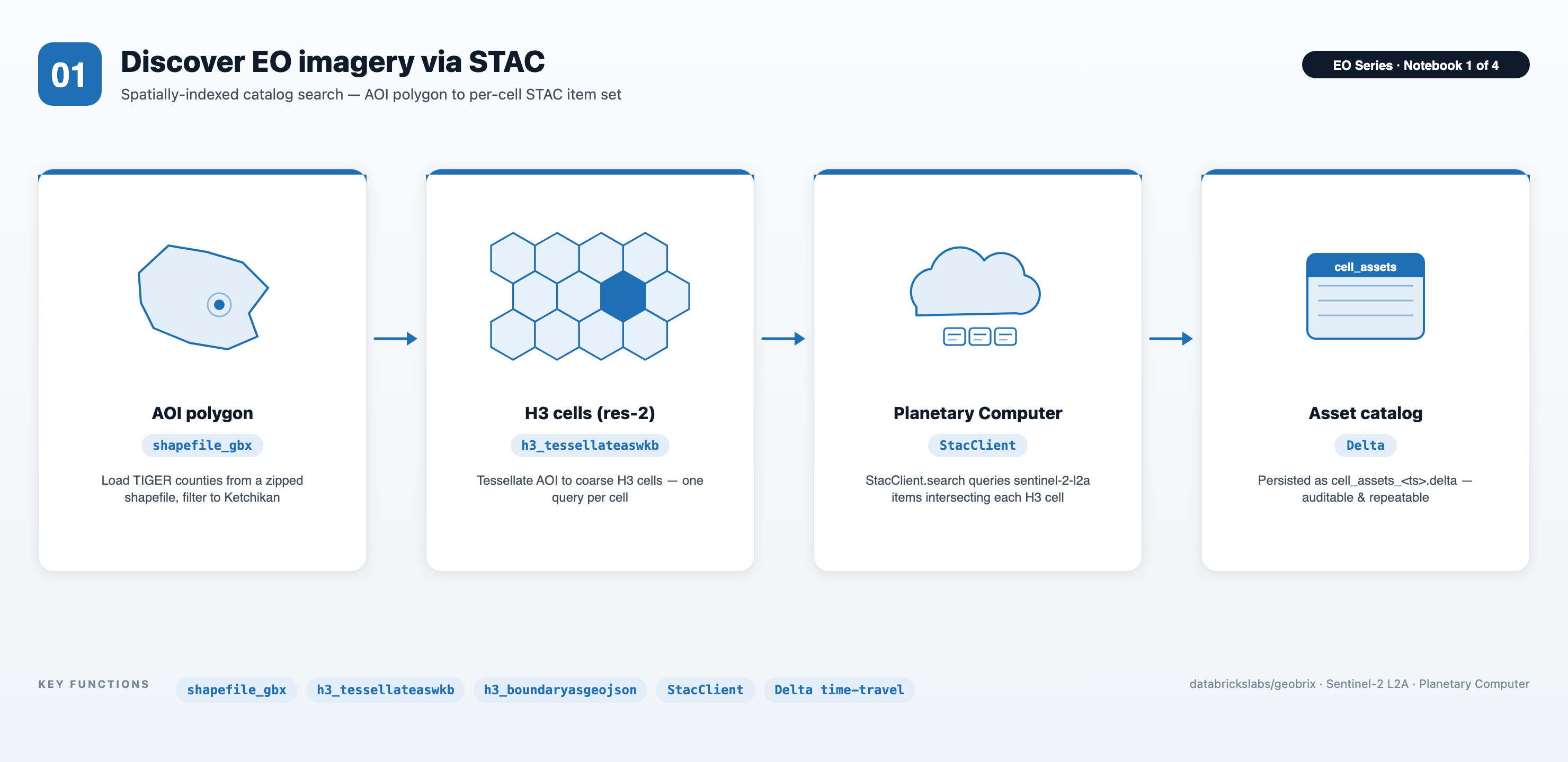
• Distributed STAC search via StacClient — tessellate any AOI polygon to H3 res-2 cells and call stac_client.search(df_cells, geojson_col="geojson", collections=["sentinel-2-l2a"], ...), which fans out one search task per cell across the cluster. Results arrive flat: one row per (cell, item, asset), pre-keyed to the grid you'll join on later.
• Shapefile I/O without unzipping — the shapefile_gbx reader pulls TIGER counties straight from a .zip blob in the Volume; no scratch-disk shuffling required.
• Persisted, time-travel-friendly catalog — search results are written to a timestamped Delta directory, giving an auditable handoff into notebook 02.

02 — Resilient band download and repair

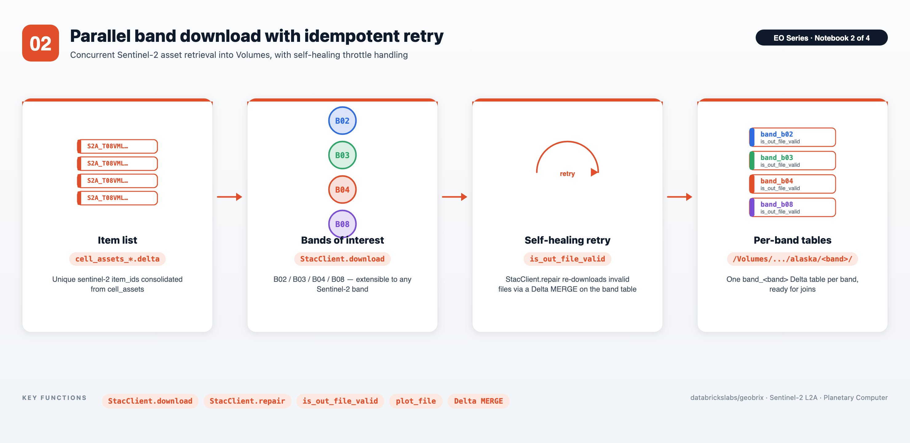
• Distributed download via StacClient — stac_client.download(band_rows, out_dir, asset_names=[band], ...) fans out one task per unique (item_id, asset_name), writing each GeoTIFF to a Volume and returning out_file_path, out_file_sz, and is_out_file_valid per file.
• Resilient and self-healing — the client re-signs URLs on every retry, validates each file with a rasterio window read (rejecting throttled error bodies and truncated files), and publishes to the Volume only when the file passes. Calling stac_client.repair("band_b02") re-downloads invalid rows and merges the results back via Delta MERGE.
• Cleanly bounded scope — only the bands you ask for (B02 / B03 / B04 / B08 by default) are pulled; the same flow extends to any other Sentinel-2 band.

03 — Tessellate rasters to H3 cells

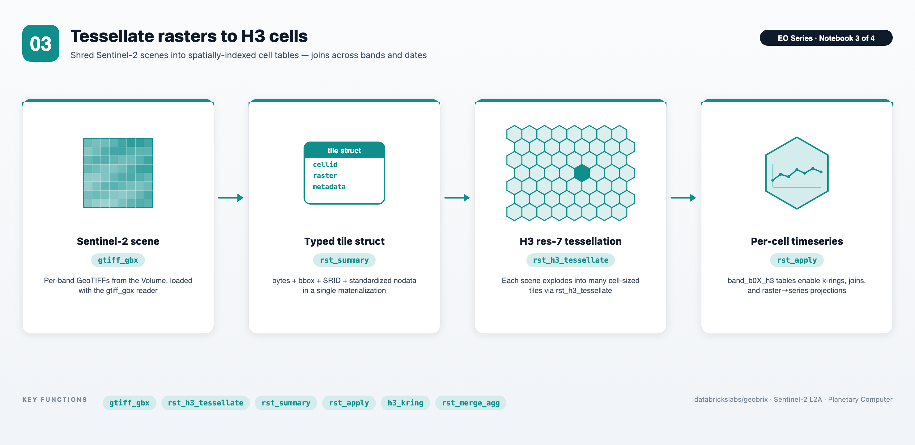
• One-step raster ingestion — the gtiff reader (and the binaryFile → rst_fromcontent pattern) materializes a typed tile column with bytes, bbox, SRID, and standardized nodata in a single pass.
• Spatial-indexed raster tables — rst_h3_tessellate shreds each Sentinel-2 scene into H3 resolution-7 cells, producing band_b0X_h3 Delta tables that join cleanly across bands and dates.
• Raster analytics from SQL/PySpark — rst_summary for per-tile stats, h3_kring + rst_merge_agg for spatial neighborhoods, and the rst_apply escape-hatch for raster-to-timeseries projection — no driver-side rasterio loops.

04 — Band Stacking + Clipping

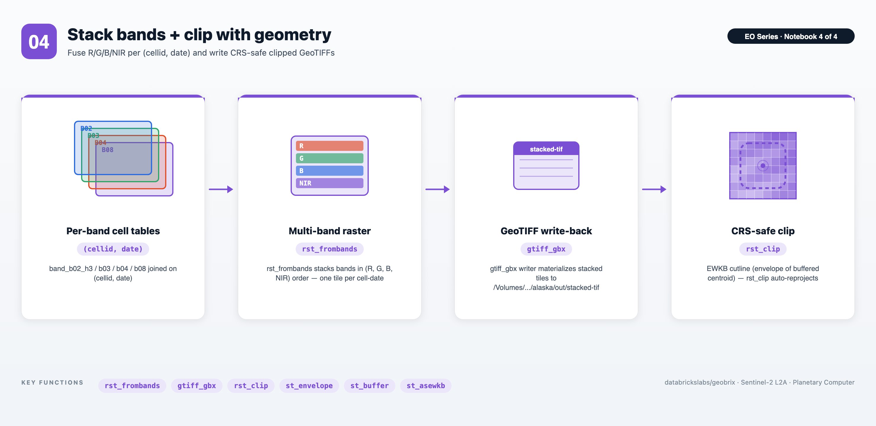
• Multi-band assembly from grid joins — joins band_b02_h3 / b03 / b04 / b08 on (cellid, date), then rst_frombands produces a single 4-band (R, G, B, NIR) tile per cell-date.
• Round-trip GeoTIFF writes — the gtiff writer (nameCol, mode("append"), option("ext", "tif")) materializes the stacked rasters back to disk in a Volume, ready for downstream tools.
• CRS-safe geometry clipping — clip cutlines built from st_envelope / st_buffer are passed as EWKB with embedded SRID, and rst_clip reprojects automatically — no per-tile CRS bookkeeping.

---

Files

File	Purpose
config_nb.ipynb	Shared setup (%run ./config_nb from every main notebook). Installs the geobrix[light,stac,vizx] wheel + EO deps, selects the tier (option-1 pyrx default / option-2 rasterx), registers functions + light readers/writers, imports the visualization helpers from databricks.labs.gbx.vizx (plot_raster, plot_file, as_gdf, cells_as_gdf) and the pyrx escape-hatches (rst_apply, tile_to_numpy), sets Unity Catalog catalog_name / schema_name, creates the /Volumes/<cat>/<schema>/data/alaska ETL tree, exposes the FORCE_REBUILD toggle and the Serverless-safe set_conf_safe() helper, instantiates stac_client = StacClient(), and defines tiling helpers (finalize_tiled_band_tbl, gen_tessellate_tiled_band).
01. Search STACs.ipynb	Loads the TIGER US Counties shapefile via the shapefile_gbx reader, filters to Ketchikan, tessellates into H3 resolution-2 cells, converts each cell to GeoJSON, and calls stac_client.search(df_cells, geojson_col="geojson", collections=["sentinel-2-l2a"], ...) to fan out per-cell queries to Planetary Computer. Writes the resulting STAC asset metadata — one row per (cell, item, asset) — to a timestamped Delta directory (cell_assets_<ts>.delta).
02. Download STACs.ipynb	Reads cell_assets_*.delta and calls stac_client.download(band_rows, out_dir, asset_names=[band], ...) for each band. Creates one band_<band> Delta table per band with item_id, band_name, date, out_file_path, out_file_sz, and is_out_file_valid columns. Calls stac_client.repair("band_<band>") to re-download and merge any files that failed read-validation.
03. Gridded EO Data.ipynb	For each band, joins the Delta band table with the gtiff reader, materializes band_<band>_tile (adds size, bbox, srid, and standardized nodata), then tessellates each tile to H3 resolution 7 into band_<band>_h3. Demonstrates rst_summary, bounding-box reprojection, h3_kring with rst_merge_agg, and raster → timeseries projection via the rst_apply escape-hatch.
04. Band Stacking + Clipping.ipynb	Joins the four band_<band>_h3 tables on (cellid, date), stacks bands in (R, G, B, NIR) order with rst_frombands into the band_stack table, writes multi-band TIFs back out via the gtiff writer (nameCol-driven filenames), and demonstrates per-tile clipping with rst_clip using a centroid-envelope buffer built from Databricks built-in ST functions.

---

Prerequisites

• Databricks Runtime 17.3 LTS / 18 LTS, or Serverless (Scala 2.13 / Spark 4 / Python 3.12). The lightweight default runs on Serverless; the heavyweight tweak needs a classic x86 cluster.
• GeoBrix (version 0.4.0). config_nb.ipynb %pip-installs the geobrix[light,stac,vizx] wheel — pure-Python bindings + rasterio + the STAC client dependencies (pystac-client, planetary-computer, tenacity, requests) + the visualization extras (matplotlib, geopandas, mapclassify) — nothing is assumed pre-staged. For the heavyweight tweak, flip option-2 (rasterx) in config_nb.ipynb and attach the GeoBrix JAR + GDAL init script to the cluster.
• Unity Catalog: edit config_nb.ipynb to set catalog_name and schema_name to your own locations. A Volume named data must already exist under <catalog>/<schema>. The notebooks create a schema if missing but will not create the Volume for you.
• Compute sizing: the lightweight default runs on Serverless. On classic clusters, the captured heavyweight runs used AWS m5d.xlarge (2–16 workers) for search/download and r6id.2xlarge (20 workers) for raster processing; an x86 instance is required for the GDAL natives. For a single county a much smaller cluster is sufficient.

---

Run order

1. Open config_nb.ipynb, set catalog_name / schema_name, and verify the Volume exists.
2. Run notebooks in numeric order: 01 → 02 → 03 → 04. Each notebook starts with %run ./config_nb so the shared state is re-established every time.

Each notebook is safe to re-run — Delta tables use do_overwrite=False / do_append=False by default, and StacClient.download skips assets whose files already exist and passed read-validation. To force a full rebuild of a notebook's outputs (re-run every step regardless of existing tables/files), set FORCE_REBUILD = True in a cell right after %run ./config_nb; it feeds the existing do_overwrite / skip-guards.

---

Data flow

TIGER shapefile (shapefile_gbx reader)
        │
        ▼  Ketchikan polygon → H3 res-2 cells → GeoJSON
STAC search (Planetary Computer, sentinel-2-l2a)
        │
        ▼  cell_assets_<ts>.delta      (nb 01)
Per-band asset download
        │
        ▼  band_b02, band_b03, band_b04, band_b08  (nb 02)
gtiff read + tile metadata
        │
        ▼  band_b0X_tile                (nb 03)
H3 tessellation @ resolution 7
        │
        ▼  band_b0X_h3                  (nb 03)
Join on (cellid, date) + rst_frombands
        │
        ▼  band_stack                   (nb 04)
gtiff writer → stacked TIFs + rst_clip
        │
        ▼  /Volumes/.../alaska/out/stacked-tif

---

Key GeoBrix / Databricks functions shown

• GeoBrix STAC (StacClient): search, download, repair — distributed STAC catalog search, resilient validated download, and Delta MERGE repair.
• GeoBrix RasterX (rx.rst_*): rst_h3_tessellate, rst_h3_tessellateexplode, rst_memsize, rst_initnodata, rst_boundingbox, rst_srid, rst_tryopen, rst_summary, rst_metadata, rst_numbands, rst_frombands, rst_fromcontent, rst_merge_agg (aggregator), rst_clip, rst_isempty.
• GeoBrix readers/writers: shapefile_gbx (zipped shapefiles without unzipping), gtiff_gbx (GeoTIFF reader + writer; the writer takes an exact (source, tile) schema with nameCol for deterministic filenames), binaryFile → rst_fromcontent pattern.
• Databricks built-in ST / H3 (DBF.*): st_geomfromwkt, st_transform, st_buffer, st_simplify, st_astext, st_asgeojson, st_aswkb, st_asewkb, st_centroid, st_envelope, h3_tessellateaswkb, h3_boundaryasgeojson, h3_boundaryaswkt, h3_toparent, h3_kring.

---

Gotchas

• Antimeridian: Alaska straddles the 180° meridian, so interactive map renderings can show results on both sides of the map.
• SRID awareness: Sentinel-2 tiles arrive in UTM zones (e.g. 32608, 32609), not EPSG:4326 — reproject bboxes before plotting on a web map.
• Free-tier auth-failure payloads: Planetary Computer returns a ~550-byte XML error body when SAS tokens expire or rate limits hit. StacClient.download validates each file with a rasterio window read, so these truncated/error responses are caught and marked is_out_file_valid = false. Call stac_client.repair("band_b02") to re-download and merge the repaired rows.
• Shuffle partitioning (Serverless-guarded): StacClient.search and StacClient.download control parallelism via partitions=; for your own steps use DataFrame.repartition(N, "col") — hash by a column, since on Serverless a number-only repartition(N) (round-robin) is coalesced by AQE back toward one partition (= serial). Any Spark-conf tuning in the notebooks goes through set_conf_safe(), which no-ops on Serverless (runtime Spark-conf mutation is disallowed there) and applies on classic clusters.
• Prefer EWKB for rst_clip cutlines: notebook 04 uses DBF.st_asewkb(DBF.st_envelope("buffer")) so the cutline's SRID travels with the bytes into rst_clip. Plain WKB (no SRID) is assumed to already be in the raster's CRS and is not reprojected; EWKB (or EWKT) with a valid SRID triggers reprojection when it differs from the raster CRS. Use st_asewkb / st_asewkt for robust, CRS-agnostic clipping.
• Scalar booleans pass through directly: rx.rst_clip("tile", "clip_wkb", True) accepts a bare Python True for the cutToCutline flag — no F.lit(True) wrapping needed.