Vapor-Eyes — Permian Methane Monitoring
Vapor-Eyes works a satellite methane signal over the Permian Basin — from a wide-area screen down to the operator whose well pad is leaking — using GeoBrix on Databricks. It comes in two flavors: a production-ready Lakeflow pipeline that can run on a schedule to stay current, and an interactive notebook series that is more of a quick start for understanding the GeoBrix functions involved in the detection cascade.
Both flavors depend on capabilities introduced in the 0.4.1 release — the netcdf_gbx reader (Sentinel-5P swath → points) and the TropomiDownloader / EmitDownloader / WellsDownloader sample downloaders — so install geobrix[light_env6,stac,vizx] 0.4.1 or newer.
- Lakeflow SDP + AI/BI Maps
- Notebook Series
A standalone, production-grade Permian Basin methane-monitoring pipeline: a Lakeflow Declarative Pipeline (SDP) plus an AI/BI dashboard, packaged as a Databricks Asset Bundle and running on the GeoBrix lightweight tier over Serverless compute.
This is the production counterpart to the notebook series (see the other tab) — same Permian AOI and satellite sources, but running on a schedule with incremental medallion tables instead of one-off notebook outputs, and a fifth data source that makes it a current (through 2026) monitoring view rather than a single historical case study.
notebooks/examples/vapor-eyes/lakeflow — the bundle, pipeline transformations, dashboard, and full setup instructions live here. See its README for deploy/run steps, prerequisites, and good-citizen usage notes for Carbon Mapper.
The pipeline and its land downloader task both install geobrix[light_env6,stac,vizx] from a staged wheel as a single pip dependency entry — pure Python/PySpark bindings (databricks.labs.gbx.pyrx, pyvx), no JAR, Serverless throughout (environment version 6). See Execution Tiers.
How it works: from a raw satellite signal to a leaderboard
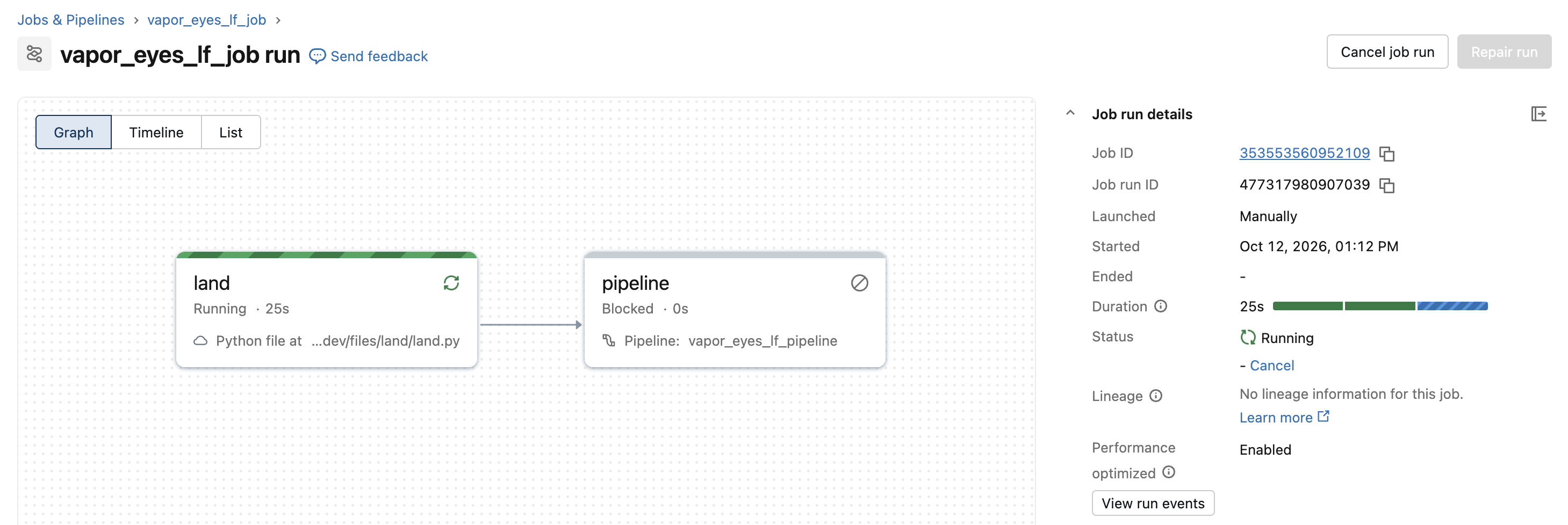
The bundle deploys one job, vapor_eyes_lf_job, with two tasks: land downloads the period's raw files, then pipeline refreshes the Lakeflow pipeline over them:
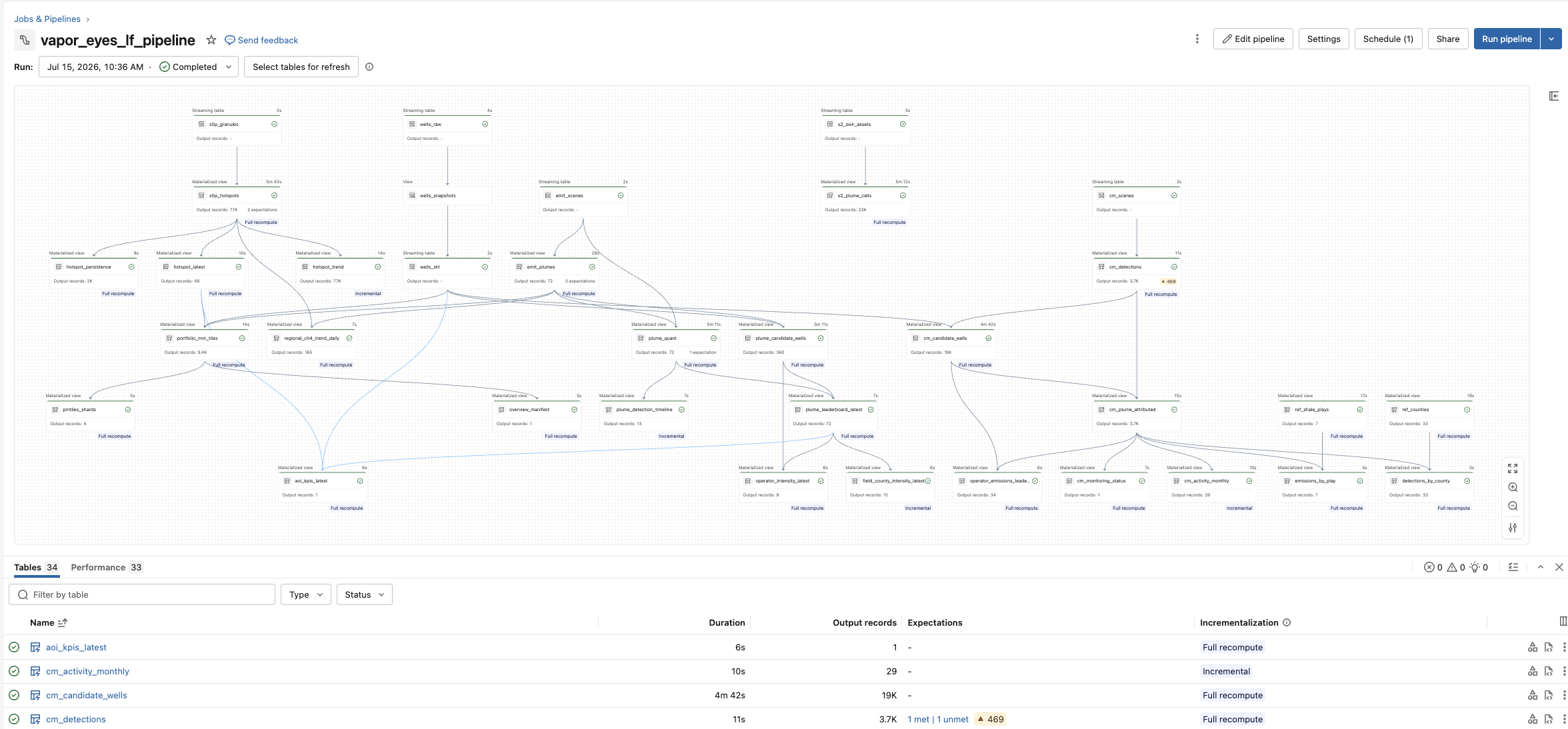
Opening the pipeline shows the lineage graph Lakeflow derived from the table-to-table dependencies, 34 tables in all. The streaming tables across the top (s5p_granules, wells_raw, s2_swir_assets, emit_scenes, cm_scenes) are the bronze inventory of what landed; the materialized views below them do the silver detection and attribution and finish in the gold tables the dashboard reads, such as plume_leaderboard_latest, operator_emissions_leaderboard, and cm_monitoring_status, with the PMTiles branch (portfolio_mvt_tiles → pmtiles_shards) alongside:
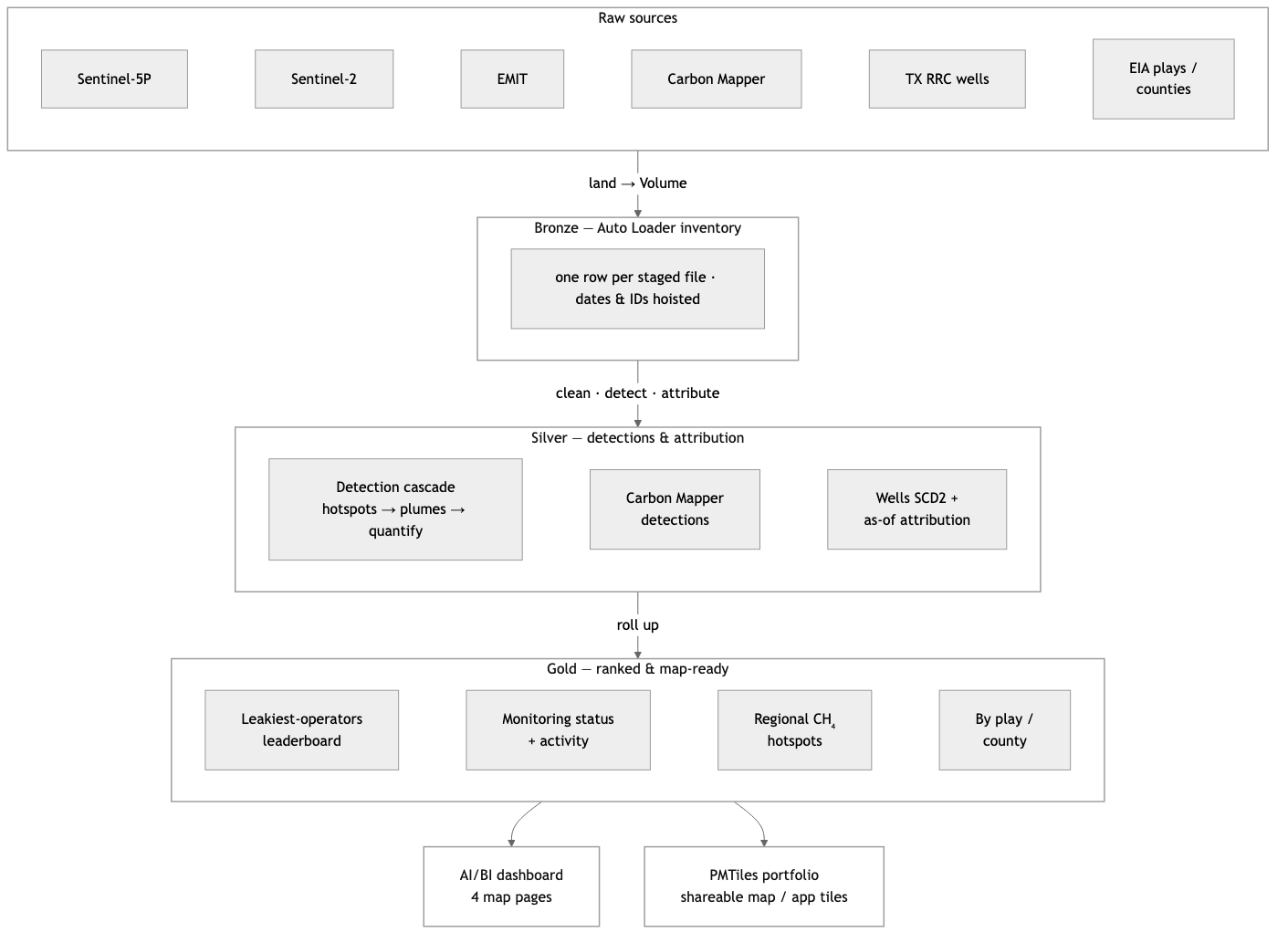
Every scheduled run turns raw satellite files into one ranked, map-ready answer — who is leaking methane in the Permian, and where — through five stages:
- Land — a downloader task pulls the period's satellite scenes, plume catalogs, and well records onto a Unity Catalog Volume.
- Bronze — what landed — Auto Loader records one row per file, lifting dates/IDs out of each filename, so re-runs pick up only new data.
- Silver — the detective work — Sentinel-5P screens the basin for CH₄ hotspots, Sentinel-2 and EMIT sharpen and quantify a plume, Carbon Mapper adds current wind-corrected detections, and each plume is tied to the operator whose well was valid on the day it was seen.
- Gold — ranked and map-ready — findings roll up into the tables the dashboard reads: the leakiest-operators leaderboard, the monitoring panel, the regional CH₄ hotspot surface, and by-play / by-county rollups.
- Serve — gold feeds the four-page AI/BI dashboard; a parallel branch folds the same findings into a self-contained PMTiles map you can drop into an app.
Each stage reads only the one before it — declared as table-to-table dependencies, so Lakeflow builds the lineage graph, orders the stages, and recomputes only what changed.
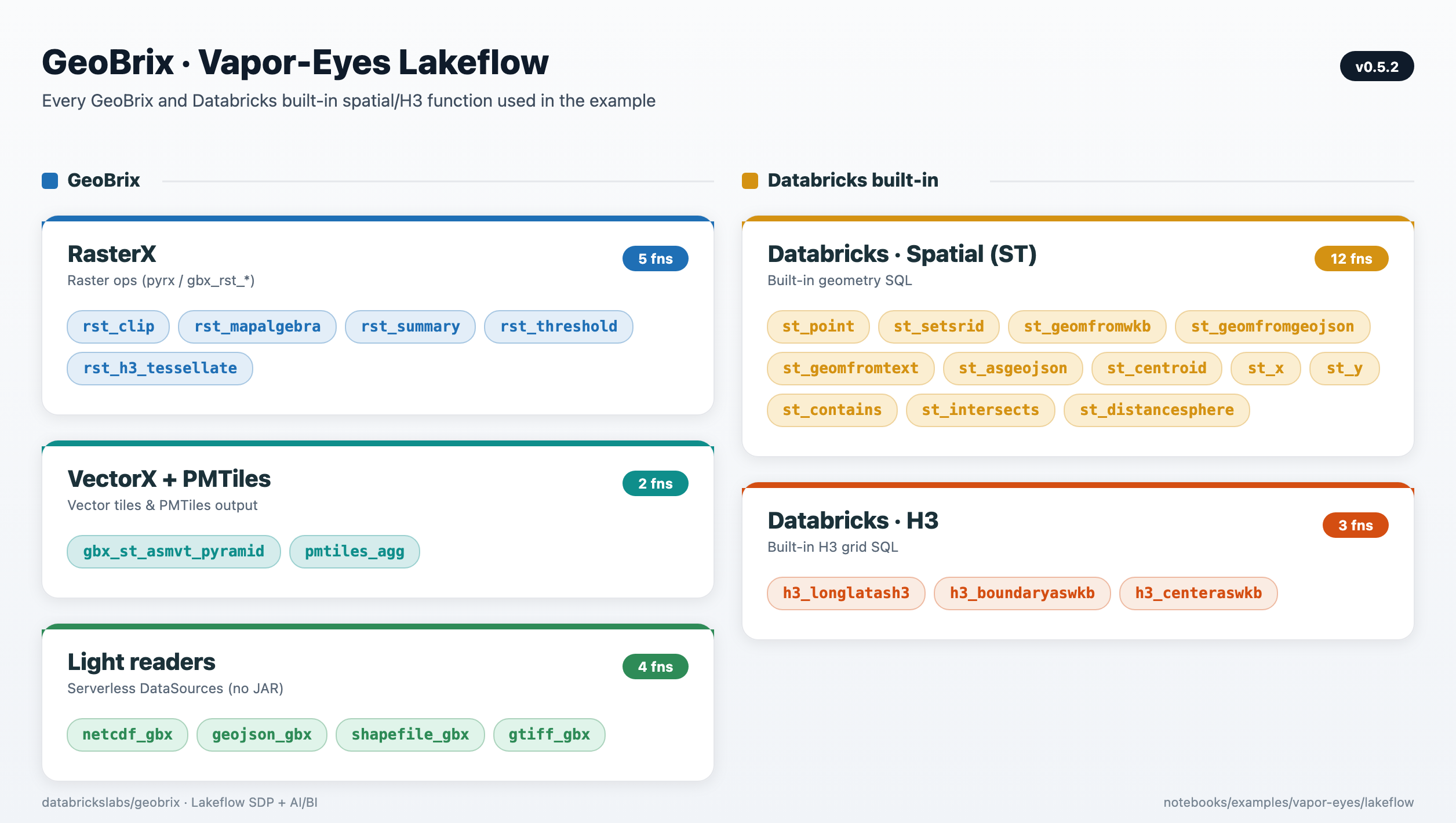
Spatial functions used
The pipeline composes GeoBrix functions with Databricks' built-in spatial SQL and H3 — RasterX for raster ops, VectorX + PMTiles for tiles, the light-tier readers for Serverless ingest, and native st_* / h3_* for geometry and gridding.
Five data sources
| Source | License | Role |
|---|---|---|
| Sentinel-5P TROPOMI | Copernicus, open | Regional CH4 screen (H3 hotspot surface) |
| Sentinel-2 SWIR | Copernicus, open | Targeted band-ratio detection at the strongest hotspot |
| EMIT | NASA LP DAAC, open (Earthdata token) | Spectral validation — GeoBrix rst_clip/rst_summary cross-check against JPL's reported concentration |
| Carbon Mapper Tanager | Carbon Mapper, public-good (free token) | The authoritative current, quantified (emission_rate_kg_hr), wind-corrected plume layer |
| TX RRC WellSHL | Public (ArcGIS REST) | Attribution — nearest-well / operator lookup |
EMIT is a science mission on the ISS with sparse revisit and roughly a 10-month lag before plume products publish, so it validates historical detections rather than driving current status. Carbon Mapper is what keeps the pipeline current: it's the only source here with a wind-corrected emission rate, and it's what the headline leaderboard and monitoring-status panels are built on.
Two small context geometries ride alongside — EIA shale plays and Census TIGER counties — read straight from source with the GeoBrix light vector reader to give the detections a "where in the basin" home.
The leaderboard, done defensibly
operator_emissions_leaderboard ranks operators by number of high-confidence Carbon Mapper plume detections, with mean/max per-detection emission rate (kg/hr) as the intensity columns — not a summed flow rate. A detection's emission_rate_kg_hr is an instantaneous rate at one overpass; summing it across a multi-year window would double-count repeat detections of the same source rather than describe a continuous flow, so the sum is retained only as a clearly-labeled secondary column, never used to rank.
cm_monitoring_status and cm_activity_monthly give the "is anything active right now" read (last detection date, plumes in the trailing 90 days, active operators) and the month-by-month activity timeline. hotspot_latest and hotspot_persistence carry the Sentinel-5P side: a current regional CH4 screen and a chronic-vs-transient emitter view.
Dashboard
Four pages, all built on AI/BI's native-geometry map widgets — H3 hexagon choropleths for the regional CH4 screen, region choropleths for the play and county rollups, and a point map for Carbon Mapper detections colored by emission rate.
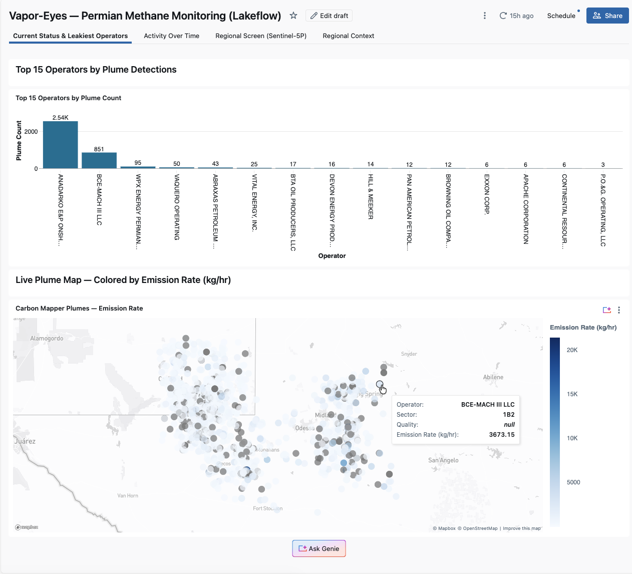
Current Status & Leakiest Operators
Monitoring-status KPIs, the operator leaderboard, and the Carbon Mapper point map with attribution.
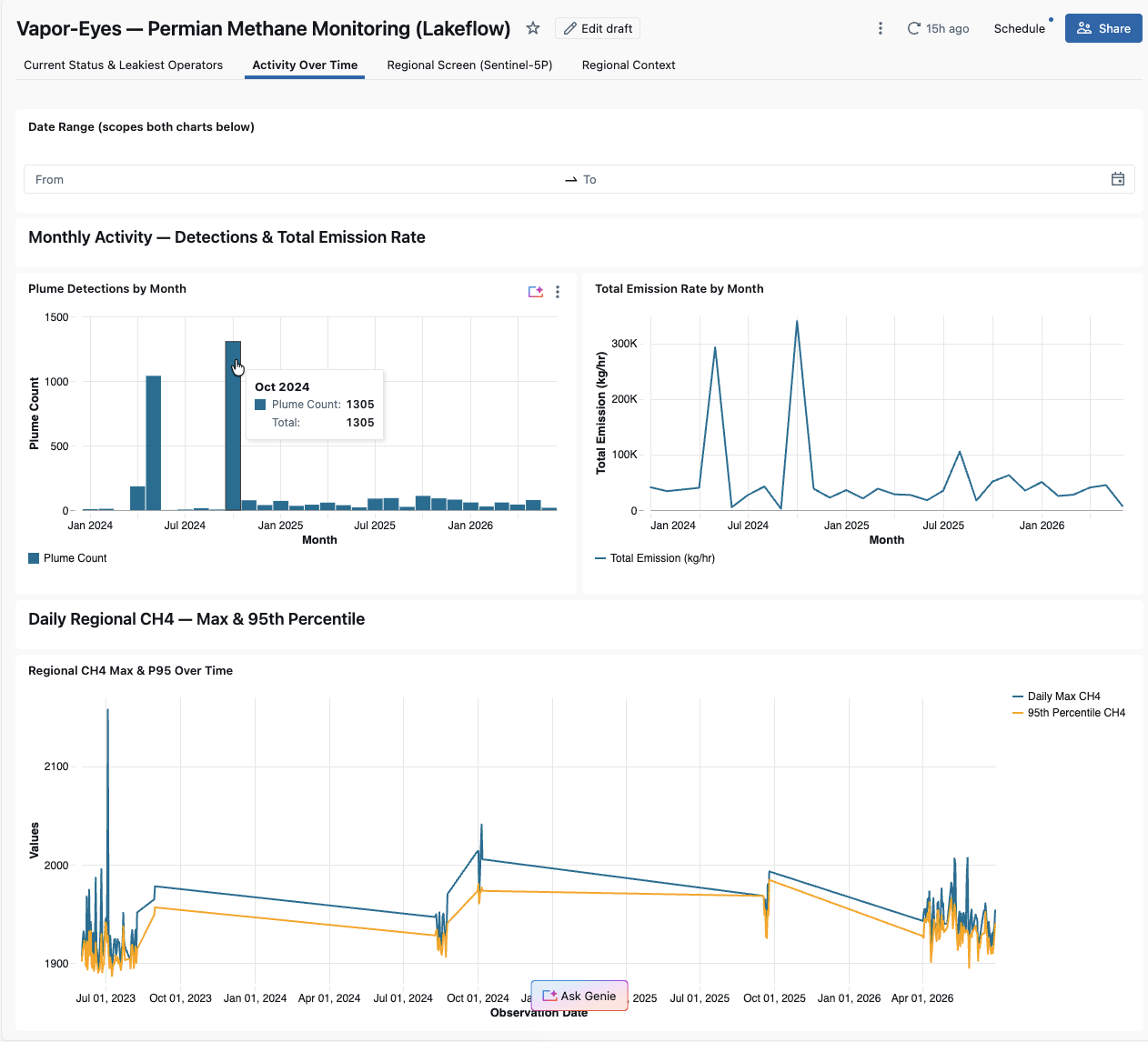
Activity Over Time
Monthly Carbon Mapper activity and the regional CH4 trend, both scoped by a shared date-range filter.
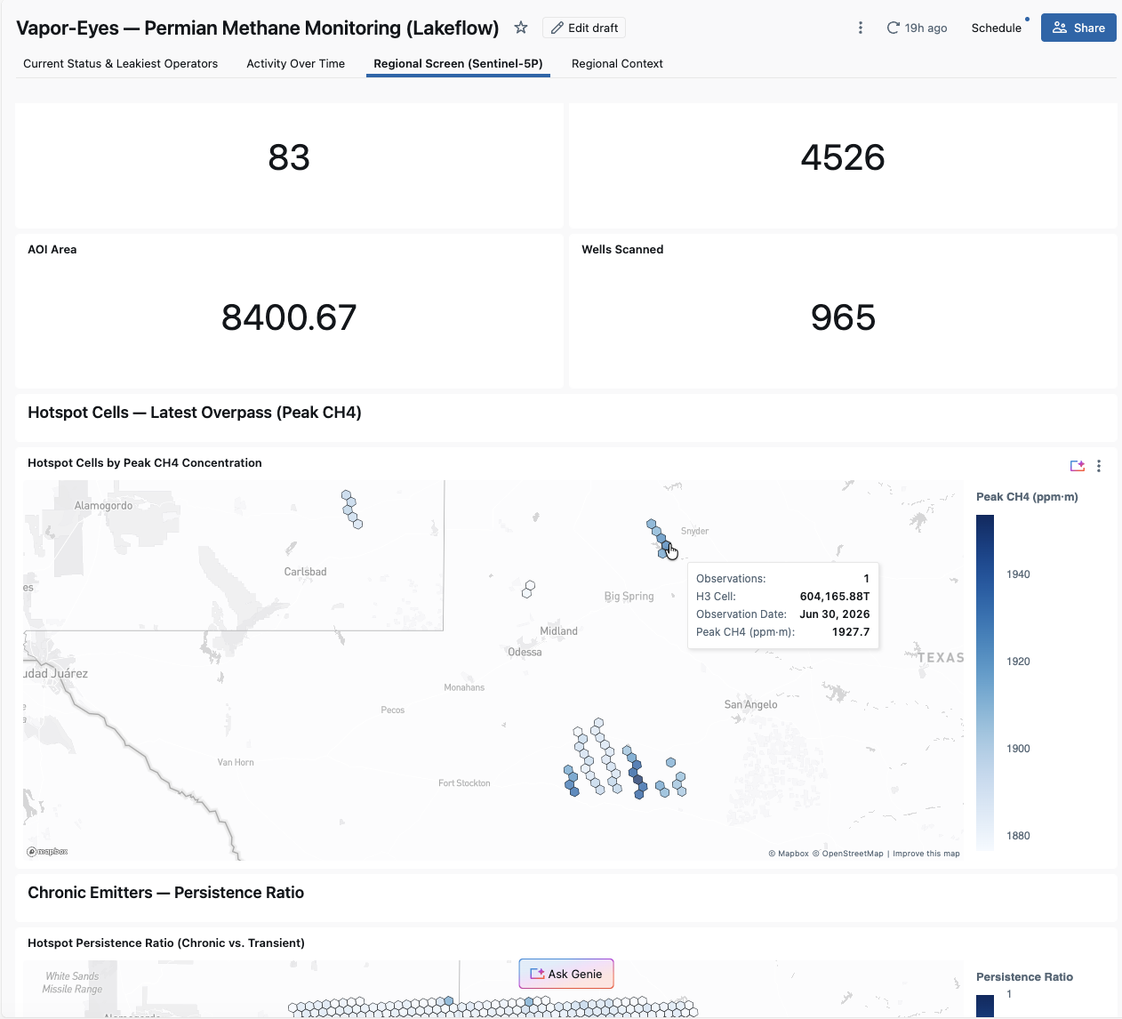
Regional Screen (Sentinel-5P)
The wide-area CH4 hotspot choropleth and the persistence choropleth.
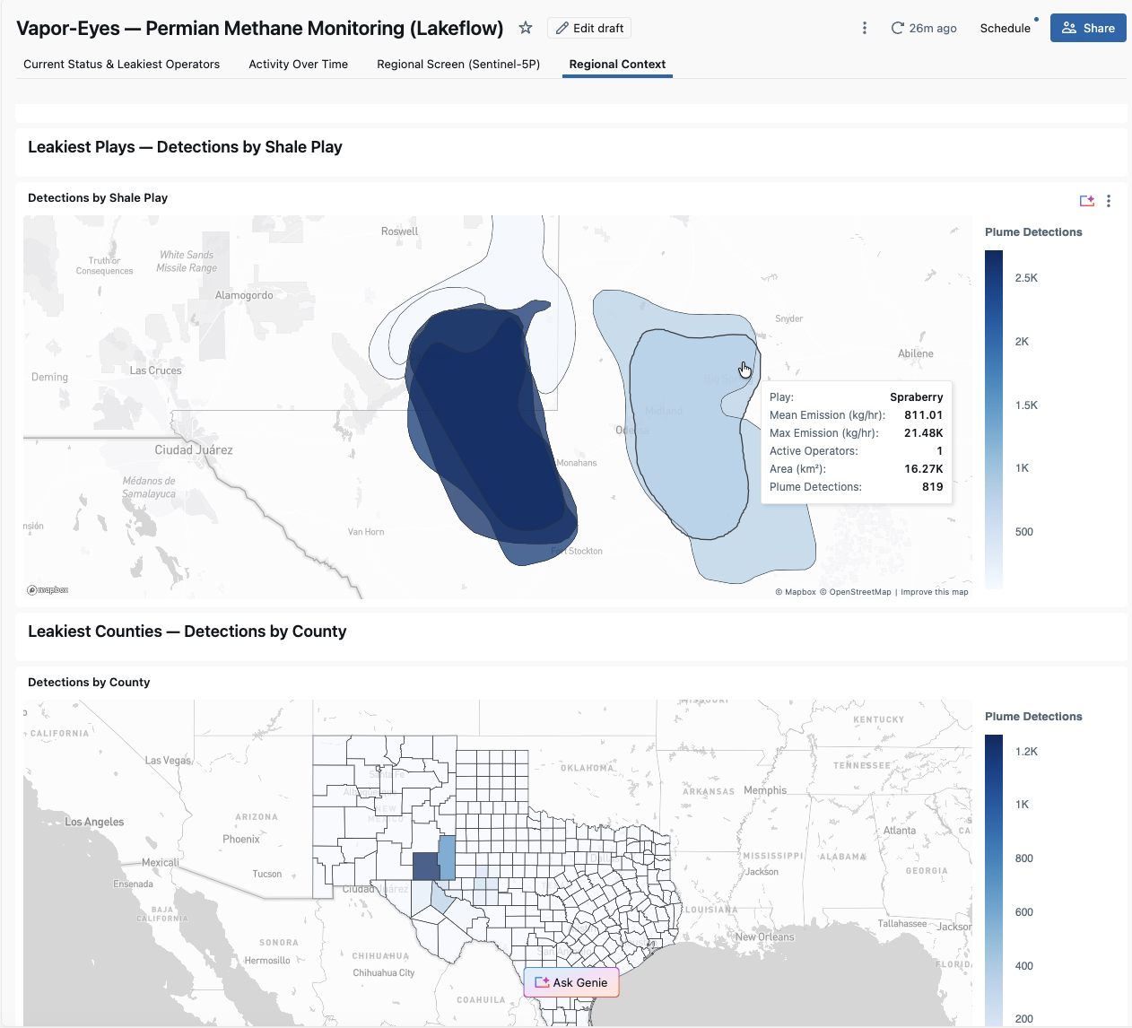
Regional Context
Carbon Mapper detections rolled up to the Permian's named shale plays (EIA) and its TX/NM counties (Census TIGER), read straight from source with the GeoBrix light vector reader and shown as two choropleths of where detections concentrate.
Good-citizen use of Carbon Mapper
Carbon Mapper's plume catalog is public-good data, and this example is built to use it responsibly: every user brings their own free token (BYOT — the pipeline is a client, not a redistributor), the dashboard shows a "Data © Carbon Mapper" attribution wherever Carbon Mapper data appears, and no Carbon Mapper data is ever committed to the repository — it's fetched at runtime straight to your own Unity Catalog Volume. This example is scoped for public-good analytics and demonstration; for commercial or low-latency operational use of Carbon Mapper/Tanager data, contact Planet Labs. See the lakeflow README for the full terms-of-use notes and token setup.
A five-notebook series that takes one Permian (Delaware Basin) bounding box and works a satellite methane signal from a wide-area screen down to a named operator's candidate well pads — then packages the whole result as a shareable PMTiles map. Each tier narrows and sharpens the last, composing GeoBrix functions with Databricks-native st_* / h3_* spatial SQL.
notebooks/examples/vapor-eyes — the five notebooks, shared config_nb, and full prerequisites live here. This is an interactive, historical case study you step through cell by cell; the other tab is the scheduled production version.
Pure Python/PySpark bindings (databricks.labs.gbx.pyrx, pyvx) plus the geobrix[light_env6,stac,vizx] wheel — no JAR. It features the net-new netcdf_gbx reader (databricks.labs.gbx.ds), which transcodes the Sentinel-5P netCDF-4 swath directly to points with no regridding. See Execution Tiers.
01 — Wide-area screening (Sentinel-5P)
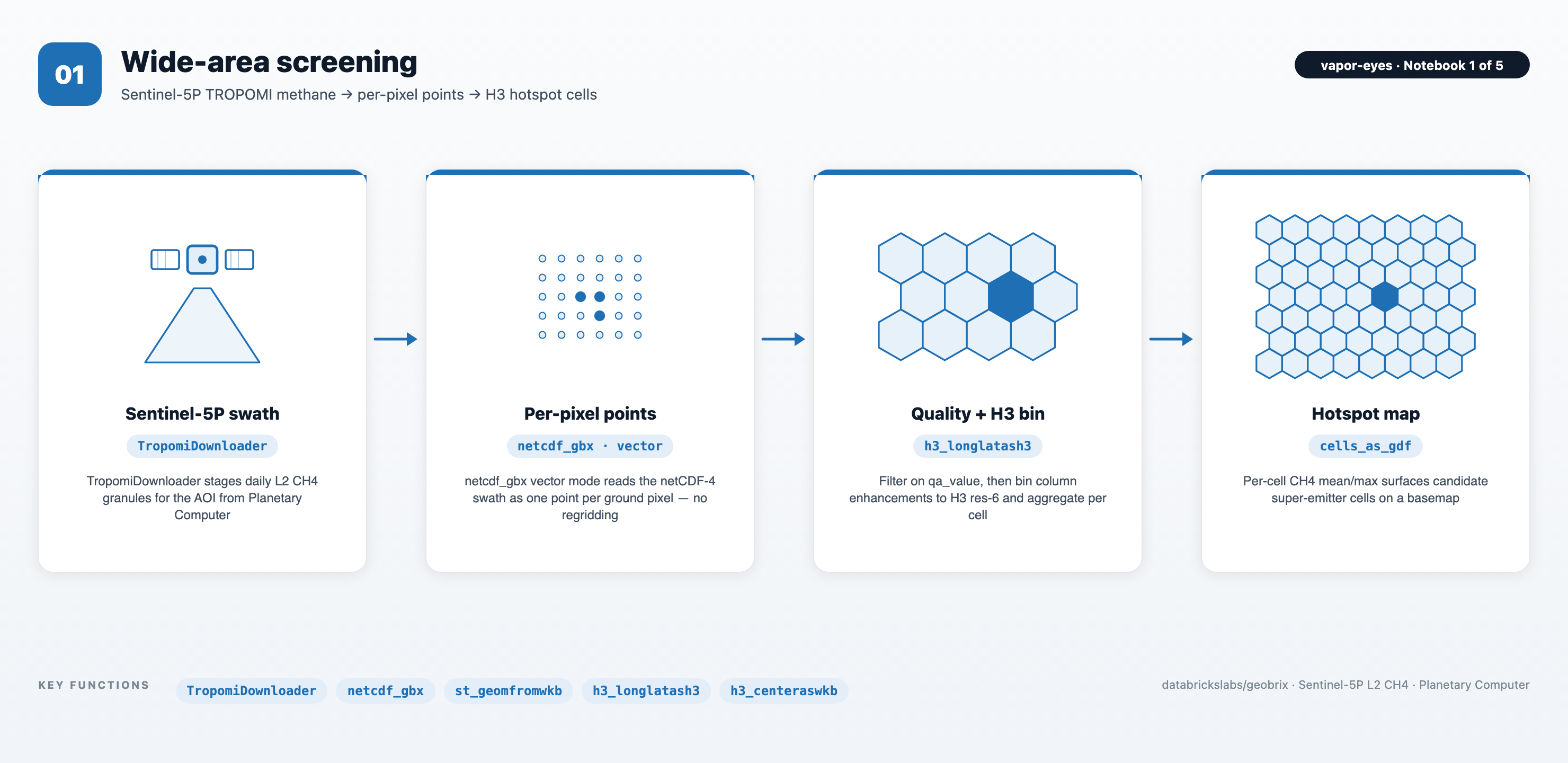
The netcdf_gbx reader transcodes each Sentinel-5P L2 CH4 granule to one point per ground pixel (no regridding, qa_value passed through); h3_longlatash3 bins pixels into res-6 cells aggregated to per-cell CH4 mean/max — the candidate super-emitter surface. The strongest cell feeds NB02.
02 — Targeted detection (Sentinel-2 SWIR)
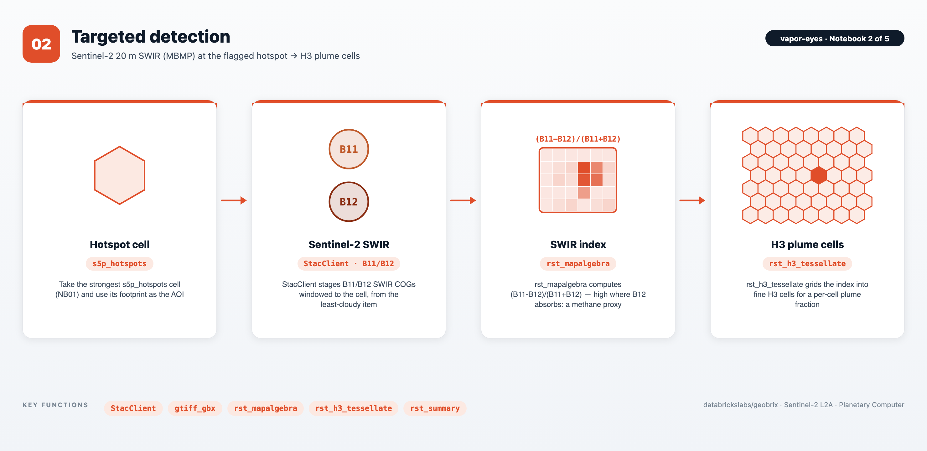
StacClient pulls the least-cloudy Sentinel-2 scene over the hotspot and downloads the B11/B12 SWIR assets windowed to the cell; gbx_rst_mapalgebra computes the (B11 − B12)/(B11 + B12) SWIR proxy and gbx_rst_h3_tessellate shreds it into fine H3 plume cells. (Illustrative proxy, not an operational retrieval — EMIT is the purpose-built instrument.)
03 — Quantification (EMIT)
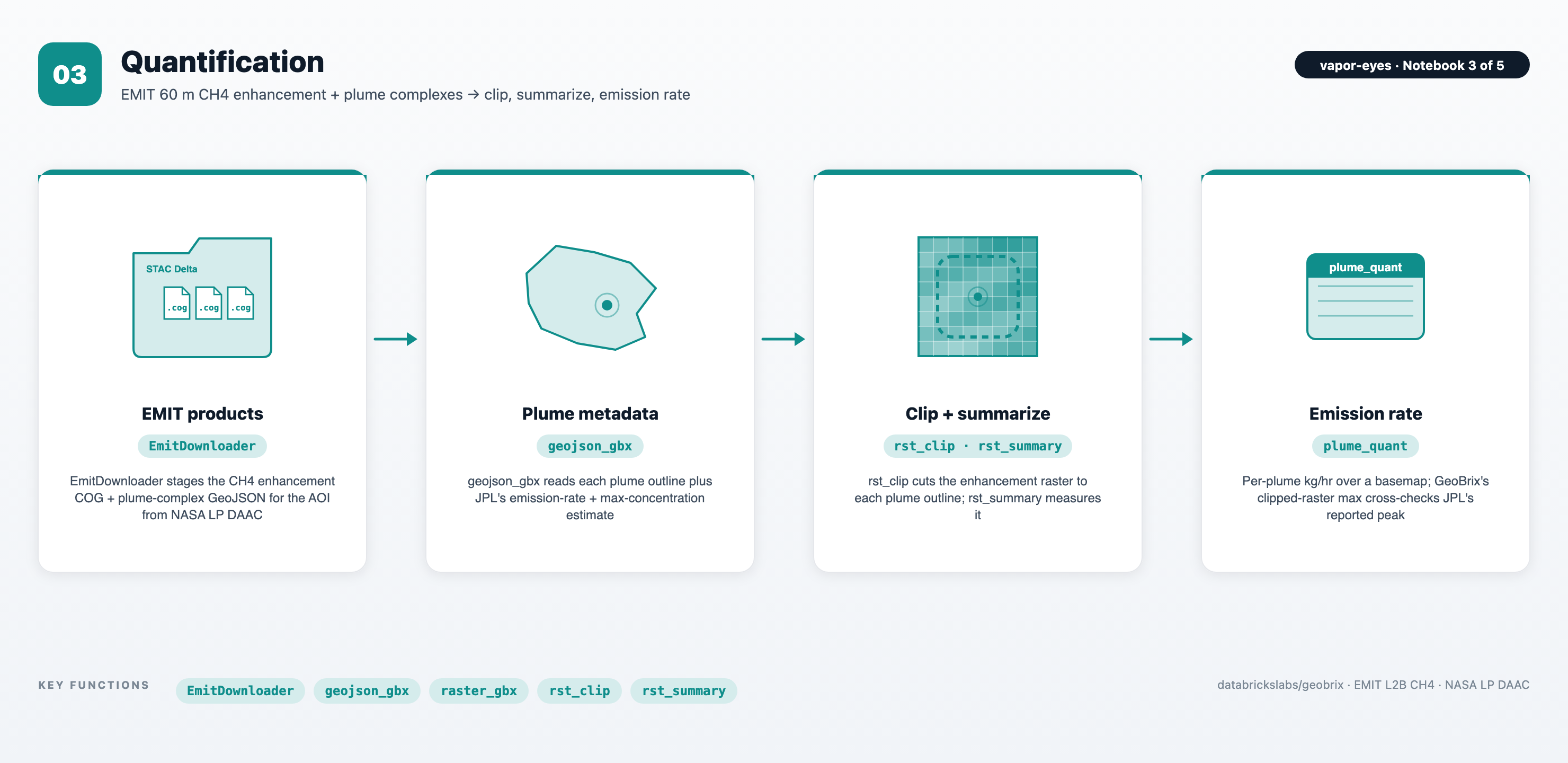
EmitDownloader stages the EMIT L2B CH4 enhancement COG and plume-complex GeoJSON (Earthdata-authenticated); gbx_rst_clip cuts the raster to each plume outline and gbx_rst_summary measures it — GeoBrix's clipped-raster max reproduces JPL's reported max concentration, an independent cross-check on real product data.
04 — Attribution (TX RRC wells)
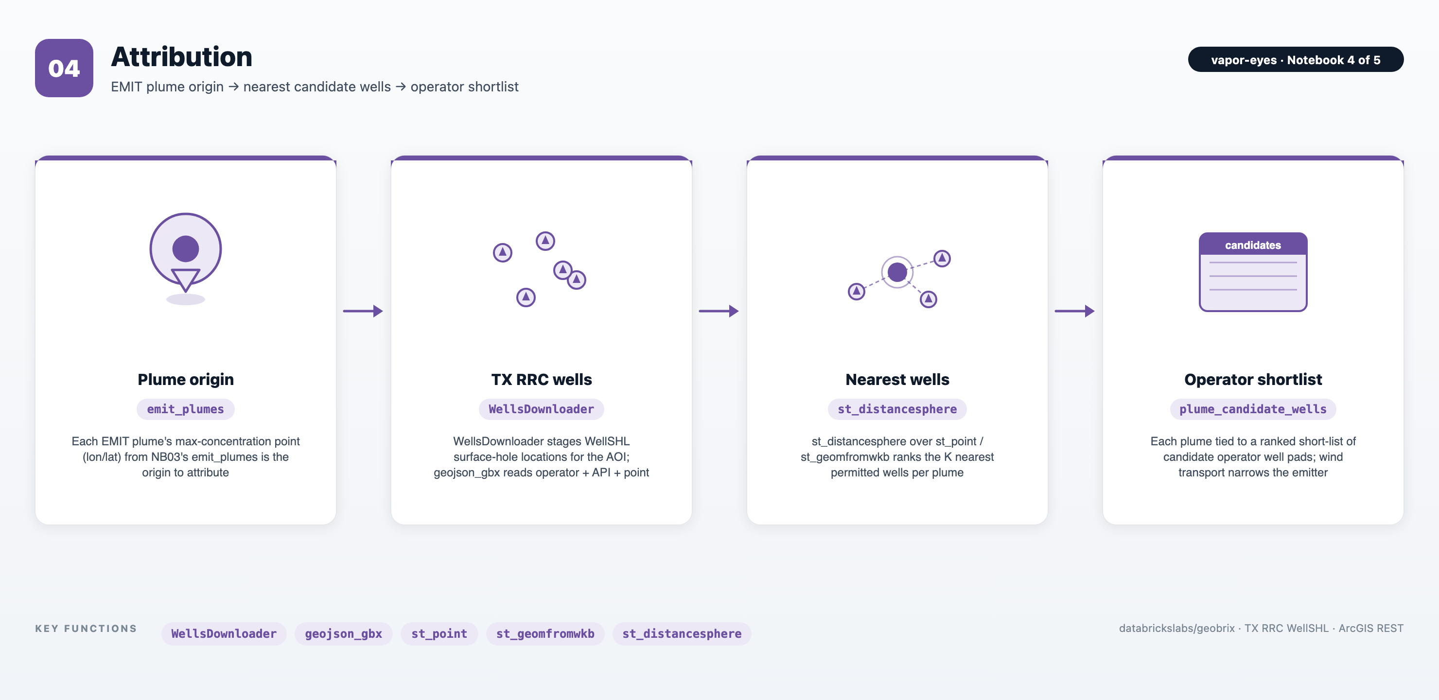
WellsDownloader pages the open TX RRC WellSHL service for wells in the AOI; st_distancesphere ranks the K nearest candidate wells per plume via a window function, tying each plume to a short-list of candidate operator well pads. (Wind transport, not proximity alone, narrows the true super-emitter.)
05 — Synthesis (vector PMTiles portfolio)
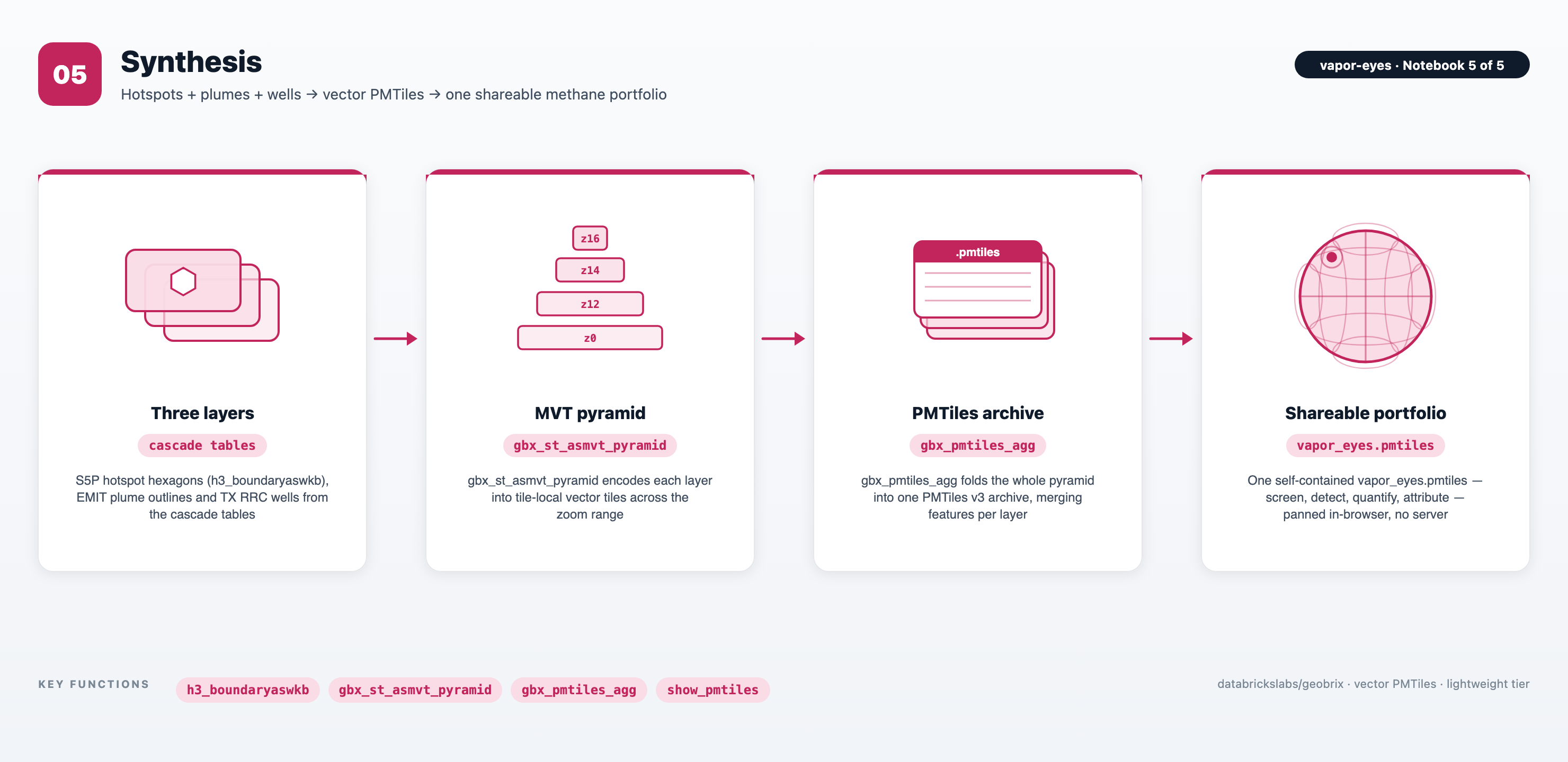
The cascade's three layers — S5P hotspot hexagons, EMIT plume outlines, and TX RRC wells — are encoded into tile-local Mapbox Vector Tiles by the gbx_st_asmvt_pyramid UDTF across a basin-to-local zoom range, then folded by gbx_pmtiles_agg into a single vapor_eyes.pmtiles v3 archive — a self-contained methane portfolio anyone can pan and zoom in a browser, no tile server.