Orthomosaic Photogrammetry — Drone Survey to Georeferenced Map
A notebook series that takes a raw drone image dataset end-to-end through EXIF/GPS telemetry extraction, quality screening, Structure-from-Motion (SfM) reconstruction, georeferenced orthomosaic production, and object + land-cover classification — from individual JPEGs to a cloud-optimized GeoTIFF ready for tile serving, and on to georeferenced object polygons and a land-cover region map. Sparse reconstruction runs on CPU; an optional dense pass and the object-segmentation part of the capstone run on GPU (land cover runs on CPU).
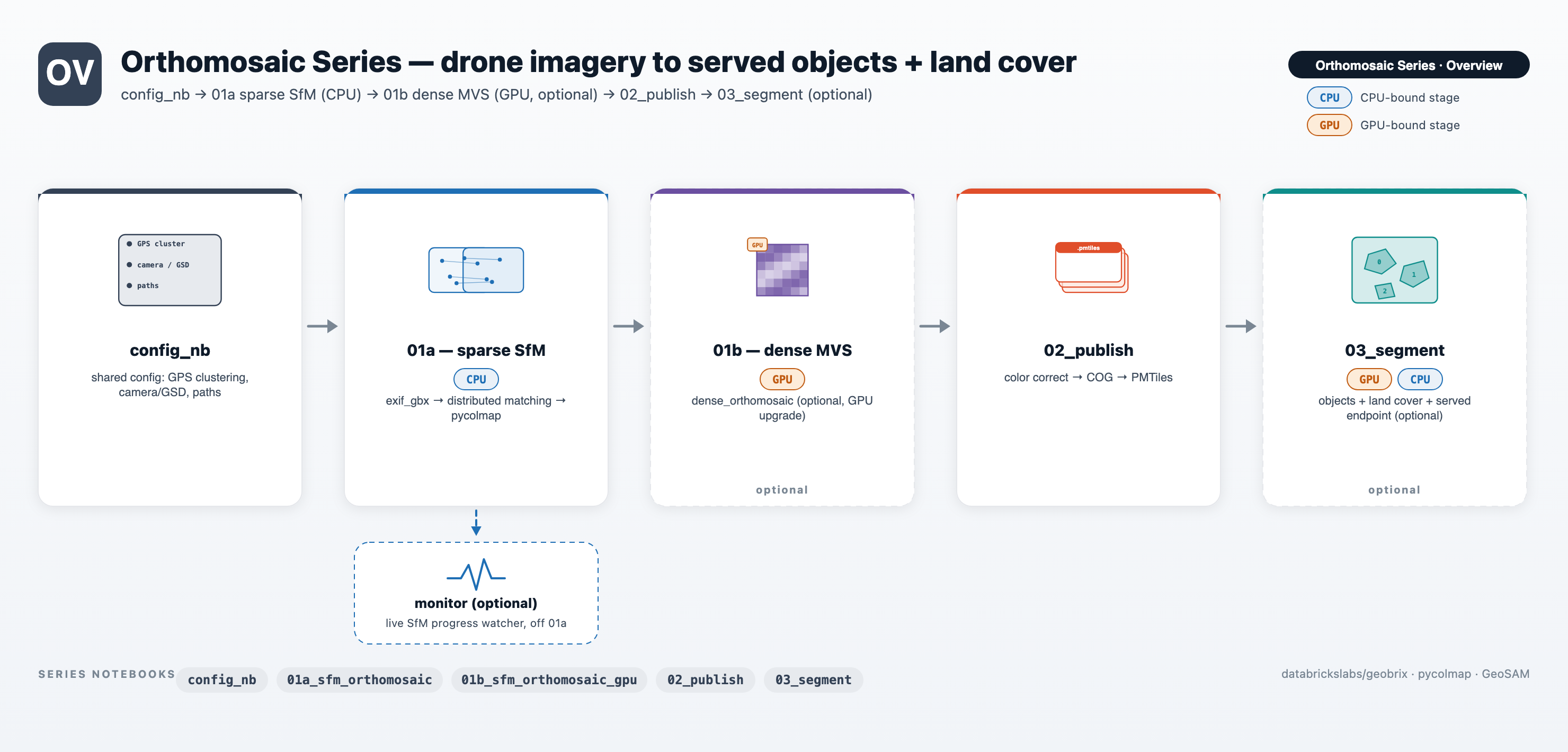
The pipeline reads EXIF metadata and GPS telemetry per-image with the GeoBrix exif_gbx
reader, computes per-image GSD and (optionally) sharpness metrics, then runs incremental
SfM with pycolmap on a Serverless environment 5 (CPU) cluster (01a). An optional
GPU notebook (01b) adds dense MVS for a higher-fidelity orthomosaic. The orthomosaic is
written as a GeoTIFF, converted to a COG with the cog_gbx writer, and packaged as a
PMTiles archive for interactive map preview. An optional capstone notebook (03_segment)
then derives two complementary views of the published COG: georeferenced object
polygons with GeoSAM (gbx.models) — in-notebook across 1..N GPUs, or behind a served
Unity Gateway GPU Model Serving endpoint — and a land-cover region map with RasterX's
rst_land_cover, entirely on CPU. See Geospatial Models,
GeoSAM, and RasterX functions.
notebooks/examples/orthomosaic — download the folder and import the numbered notebooks into your Databricks workspace to run.
The series runs on Serverless environment 5 (Python 3.11, CPU only). Install via:
geobrix[light_env5,photogrammetry,vizx] @ file:///Volumes/.../geobrix-0.5.2-py3-none-any.whl
The photogrammetry extra brings pycolmap >= 4.0.0, rasterio, rio-cogeo, and the
PMTiles toolchain. No JAR or GDAL init script is needed.
01a runs sparse SfM on CPU. An optional dense pass (01b) runs COLMAP
patch_match_stereo on the Serverless GPU AI Runtime (pycolmap-cuda12, CUDA 12),
producing a dense orthomosaic, DSM, and LAZ point cloud. The sparse ortho alone is
suitable for GSD estimation, visual inspection, and georeferenced tile serving; the dense
pass adds fidelity for measurement workflows. 02_publish uses whichever orthomosaic is
present (dense if 01b ran, else sparse).
03_segment (optional) turns the published COG into objects AND a land-cover map. It
installs its own extras — geobrix[light_env5,models_gpu_env5,vizx] — rather than
photogrammetry, since its instance-objects section needs GeoSAM's
torch/segment-geospatial, not pycolmap, and runs on the Serverless GPU AI Runtime
(environment 5). Its land-cover section is plain RasterX (rst_land_cover, CPU-only) and
needs no GPU. The notebook is standalone (no %run ./config_nb) and can run any time after
02_publish has written orthomosaic_cog.tif.
Executed output — Old Orchard drone survey
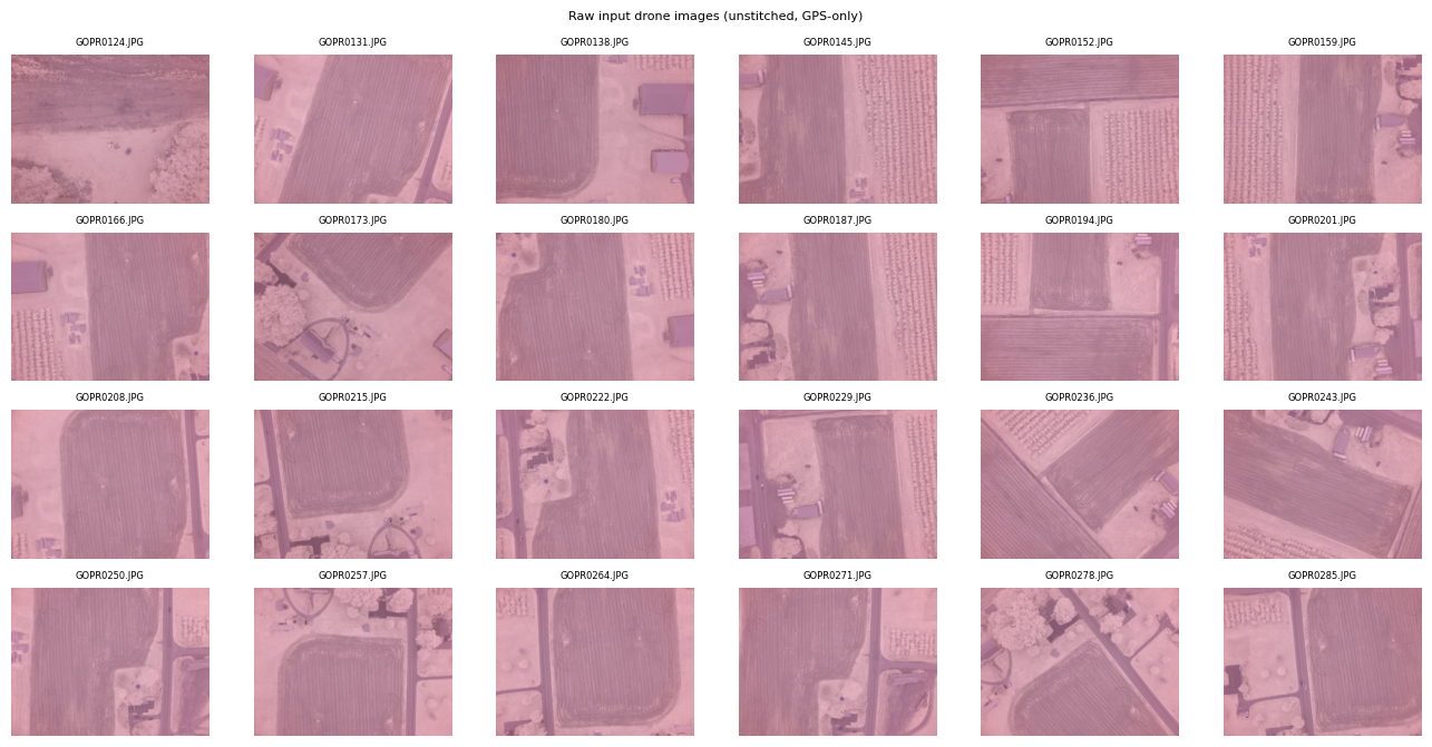
These screenshots are pulled from the executed notebook series, run over the Old Orchard GoPro survey (~170 overlapping, GPS-tagged frames) that the committed notebooks download by default.
The raw inputs: an evenly spaced contact sheet of the unstitched frames that SfM must align and stitch:
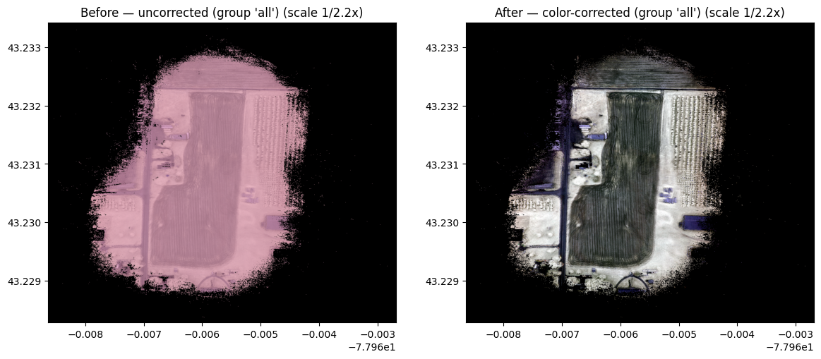
After reconstruction, Part 2 color-corrects the orthomosaic with a per-band percentile stretch, uncorrected on the left and corrected on the right:
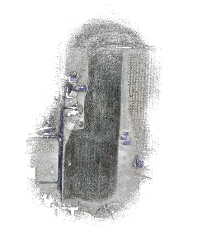
The published PMTiles archive rendered in the notebook, the same tiles a web map serves:
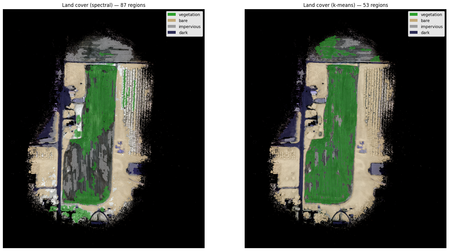
Finally, the capstone classifies the whole scene into contiguous land-cover regions (vegetation, bare, impervious, dark) with rst_land_cover, spectral thresholds beside k-means:
The notebooks
config_nb — shared configuration and helpers
Shared imports, pipeline parameters (GSD_CM, MAX_ORTHO_WORKERS, GROUP_KEY_COL),
and the SfM helper functions used by the numbered notebooks. Import once; the numbered
notebooks run %run ./config_nb.
01a_sfm_orthomosaic — telemetry → SfM → orthomosaic
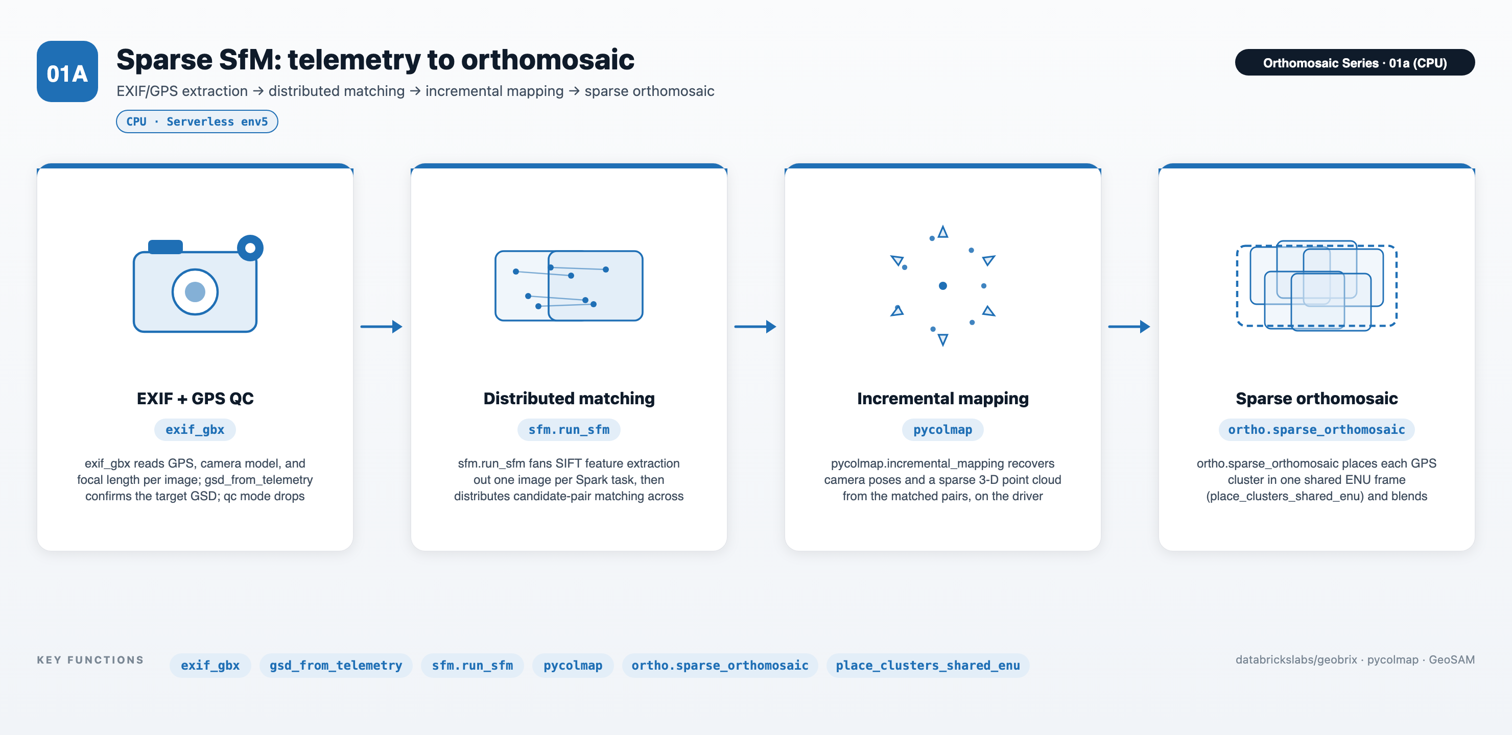
The core pipeline:
- EXIF extraction —
exif_gbxreader scans the image directory, emitting one row per image with GPS coordinates, camera model, focal length, and pixel dimensions. - GSD estimation —
gsd_from_telemetry(focal_length_mm, altitude, image_width, sensor_width_mm)computes ground sampling distance (cm/pixel) per image. - Optional QC screen — if
QC_MODE=True, re-reads withmode="qc"to appendsharpnessandbrightness; blurry images belowMIN_SHARPNESSare dropped before reconstruction. - Distributed feature extraction — SIFT features are extracted per-image as a
Spark map operation (one task per image, Serverless fan-out via
repartition). - Pair matching — exhaustive or sequential matching with
pycolmap's GPU-free CPU matcher; results are collected to the driver for the reconstruction step. - Incremental mapping —
pycolmap.incremental_mappingrecovers camera poses and a sparse 3-D point cloud on the driver. - Orthomosaic projection — each registered image is back-projected onto the estimated
ground plane; contributions are blended by overlap count into a georeferenced RGB
GeoTIFF (
orthomosaic.tif).
01b_sfm_orthomosaic_gpu (optional) — dense MVS on GPU
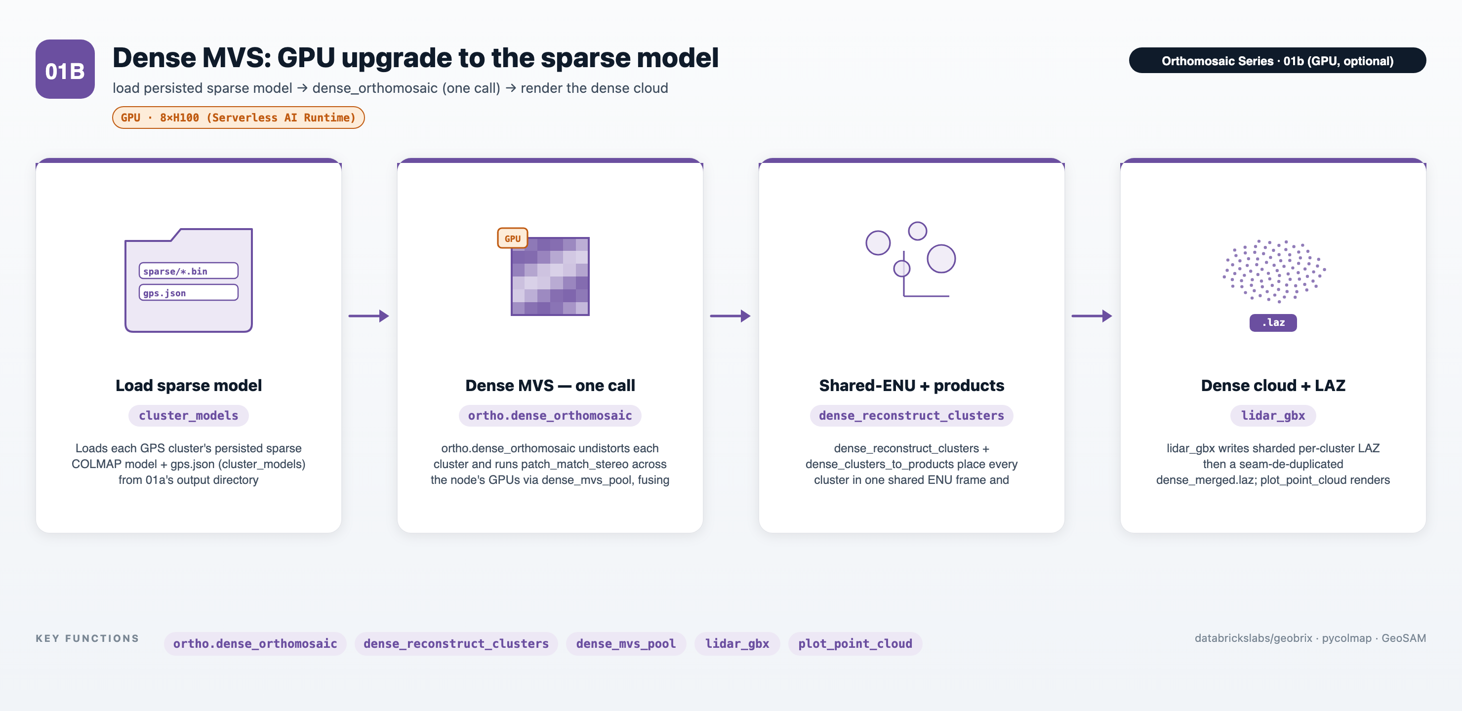
An optional GPU notebook that upgrades the sparse result to a dense reconstruction. It
loads the persisted sparse model from 01a and, per group, makes one call —
ortho.dense_orthomosaic — that reconstructs every GPS cluster (undistort, COLMAP
patch_match_stereo across the node's GPUs via a driver-side GPU-slot scheduler sized by
recommend_dense_allocation, and fuse to a per-cluster fused.ply, with per-cluster
checkpointing) and then georeferences the result into a dense RGB orthomosaic, DSM, and
LAZ point cloud (per-cluster and merged); see the pyrx.ortho module reference further
down this page for its full API. Runs on the Serverless GPU AI Runtime (environment 5,
pycolmap-cuda12, CUDA 12); 01a is the CPU peer that produces the sparse model it
consumes. 02_publish automatically uses the dense orthomosaic when present.
02_publish — color correction → COG → PMTiles
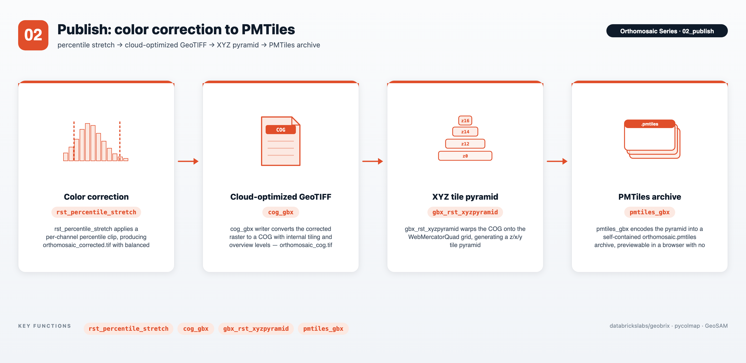
A single publish notebook that turns orthomosaic.tif into web-ready deliverables in
three checkpointed stages:
- Color correction — a per-channel percentile stretch (configurable low/high clip
percentiles) produces
orthomosaic_corrected.tifwith balanced contrast, persisted so the served COG and PMTiles carry it. - Cloud-optimized GeoTIFF — the
cog_gbxwriter converts the corrected raster to a COG with internal tiling and overview levels, producingorthomosaic_cog.tiffor efficient range-request reads downstream. - PMTiles — the COG is warped onto the WebMercatorQuad grid with
gbx_rst_xyzpyramidand encoded into a self-containedorthomosaic.pmtilesarchive by thepmtiles_gbxwriter, previewable in a browser (PMTiles + MapLibre GL or Leaflet) with no tile server.
Each stage is checkpointed per group; set FORCE_CORRECTED / FORCE_COG /
FORCE_PMTILES in config_nb to recompute a stage.
03_segment (optional) — objects + land cover capstone
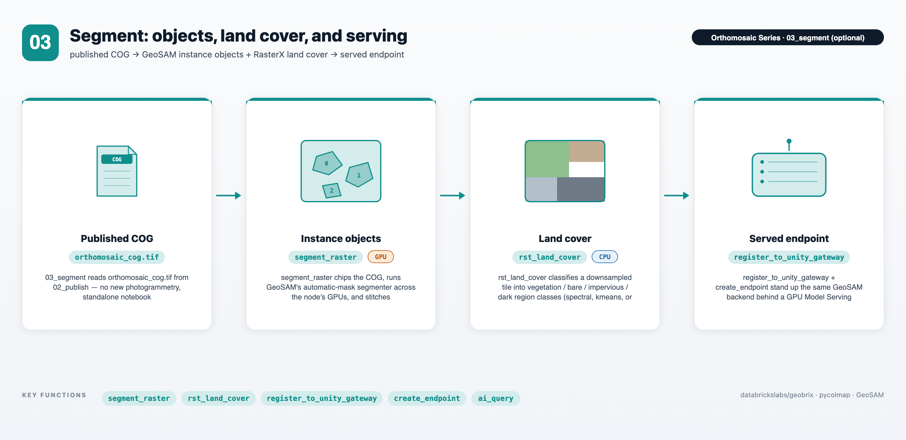
A capstone notebook that derives two complementary views of 02_publish's orthomosaic
COG — discrete objects and a land-cover region map — then serves the object model.
It runs no new photogrammetry; it only reads orthomosaic_cog.tif.
- Instance objects (GPU) — a single
segment_rastercall chips the COG into an overlapping grid, runs GeoSAM's automatic-mask segmenter across the node's GPU(s) (gpus="all"), stitches each chip's label mask into whole-object polygons using its own true per-window georeferencing, and returns apandas.DataFrameoflabel(int),geom(WKB bytes), andscore(float). Automatic-mask GeoSAM is class-agnostic (instance segmentation) — each object gets an id, not a semantic type — so the preview colors objects by instance id with a legend. - Land cover (CPU) — the complementary view: partition the whole scene into
contiguous region classes (vegetation / bare / impervious / dark) with RasterX's
rst_land_cover, composed from the existingrst_*family —rst_fromfile→rst_resample(downsample so a single tile fits worker memory) →rst_land_cover(an Int32 class-mask tile) →gbx_rst_polygonize→ labeled polygons, filtered to regions at or above a metric minimum area viacore.crs.area_m2. The notebook runs bothmethod="spectral"(fixed thresholds) andmethod="kmeans"(adaptive clustering) side by side so the two can be compared —method="hybrid"(rst_land_cover's default) is the pragmatic blend of the two. - Served endpoint — the same GeoSAM backend wrapped as an MLflow pyfunc
(
build_geosam_pyfunc), registered to the Unity Catalog model registry (register_to_unity_gateway), and stood up behind a GPU Model Serving endpoint (create_endpoint,scale_to_zero=Trueby default) for programmatic, notebook-free access.
The instance-objects section needs a GPU cluster — GeoSAM's SAM backbone is
CUDA-bound — so it runs on the Serverless GPU AI Runtime (environment 5). The
land-cover section is CPU-only RasterX and needs no GPU. The serving section
(registration, endpoint creation, querying) is API calls that can run from any cluster
with mlflow installed.
Calling the served endpoint — four ways
Once registered to Unity Catalog and served behind the Unity Gateway, the endpoint is a
standard Databricks Model Serving
REST endpoint — callable from a notebook, an app, a job, or SQL with no GeoBrix package
and no GPU attached on the calling side. All four forms below hit the same
.../serving-endpoints/geosam-ortho-endpoint/invocations URL with the same image_b64
input and get back the same shape:
{"predictions": {"geojson": "{\"type\": \"FeatureCollection\", \"features\": [{\"type\": \"Feature\", \"geometry\": {\"type\": \"Polygon\", \"coordinates\": [[[-121.9744, 36.9744], ...]]}, \"properties\": {\"label\": 0, \"score\": 1.0}}]}"}}
predictions is a dict {"geojson": ...}, not a list. The decoded geojson value
is a GeoJSON FeatureCollection string with one Polygon Feature per detected
object, carrying properties.label (int) and properties.score (float).
- curl
- Python (JSON)
- Python (protobuf)
- SQL
curl \
  -u token:$DATABRICKS_TOKEN \
  -X POST \
  -H "Content-Type: application/json" \
  -d@data.json \
  https://e2-demo-field-eng.cloud.databricks.com/serving-endpoints/geosam-ortho-endpoint/invocations
data.json holds the request body, e.g.
{"dataframe_records": [{"image_b64": "<base64 GeoTIFF tile>"}]}. The quickest smoke
test for the endpoint, and it works from any language that can shell out to curl.
import os
import requests
import numpy as np
import pandas as pd
import json

def create_tf_serving_json(data):
    return {'inputs': {name: data[name].tolist() for name in data.keys()} if isinstance(data, dict) else data.tolist()}

def score_model(dataset):
    url = 'https://e2-demo-field-eng.cloud.databricks.com/serving-endpoints/geosam-ortho-endpoint/invocations'
    headers = {'Authorization': f'Bearer {os.environ.get("DATABRICKS_TOKEN")}', 'Content-Type': 'application/json'}
    ds_dict = {'dataframe_split': dataset.to_dict(orient='split')} if isinstance(dataset, pd.DataFrame) else create_tf_serving_json(dataset)
    data_json = json.dumps(ds_dict, allow_nan=True)
    response = requests.request(method='POST', headers=headers, url=url, data=data_json)
    if response.status_code != 200:
        raise Exception(f'Request failed with status {response.status_code}, {response.text}')
    return response.json()
The dataframe_split record shape most services call Model Serving with. GeoBrix wraps
exactly this — base64-encoding the tile and posting the request — as
serving.query, so most notebook/job callers
reach for that instead of re-deriving this.
import os
import requests
import numpy as np
from tritonclient.grpc.service_pb2 import ModelInferRequest, ModelInferResponse  # KServe v2 ModelInferRequest/Response
from tritonclient.utils import np_to_triton_dtype, triton_to_np_dtype  # numpy<->KServe v2 dtype helpers

def create_kserve_request(data):
    tensors = data if isinstance(data, dict) else {'input': data}
    request = ModelInferRequest()
    for name, array in tensors.items():
        array = np.ascontiguousarray(array)
        request.inputs.add(name=name, datatype=np_to_triton_dtype(array.dtype), shape=array.shape)
        request.raw_input_contents.append(array.tobytes())
    return request

def score_model(dataset):
    url = 'https://e2-demo-field-eng.cloud.databricks.com/serving-endpoints/geosam-ortho-endpoint/invocations'
    headers = {'Authorization': f'Bearer {os.environ.get("DATABRICKS_TOKEN")}', 'Content-Type': 'application/x-protobuf'}
    request = create_kserve_request(dataset)
    response = requests.request(method='POST', headers=headers, url=url, data=request.SerializeToString())
    if response.status_code != 200:
        raise Exception(f'Request failed with status {response.status_code}, {response.text}')
    result = ModelInferResponse()
    result.ParseFromString(response.content)
    return {output.name: np.frombuffer(result.raw_output_contents[i], dtype=triton_to_np_dtype(output.datatype)).reshape(output.shape) for i, output in enumerate(result.outputs)}
The KServe v2 binary protocol (application/x-protobuf) — lower-overhead than JSON for
large tensor payloads.
SELECT ai_query('geosam-ortho-endpoint',
    request => named_struct('image_b64', <value>))
Calls the endpoint inline from SQL or a Lakeflow pipeline via
ai_query
— the columnar, at-scale path: fan segmentation out over a whole table of image
tiles with one query, no notebook or Python client involved.
See the
Unity Catalog model lifecycle
docs for how a registered, versioned model like this one is governed, and the
Serving reference page for GeoBrix's own wrappers —
serving.query, register_to_unity_gateway, build_geosam_pyfunc, and
geosam_signature — that 03_segment uses to get here.
monitor (optional) — live SfM progress
An optional utility notebook that polls the SfM working directory and prints incremental
reconstruction statistics (registered images, 3-D points) while 01a_sfm_orthomosaic runs.
Key GeoBrix functions shown
exif_gbxreader —spark.read.format("exif_gbx").option("mode", "metadata").load(path)emits one row per image with GPS coordinates, camera identity, focal length, pixel dimensions, and aPOINT WKBgeometry column.mode="qc"addssharpnessandbrightness. Options:filterRegex,sensorWidthMm,focalLengthMm. See EXIF/GPS reader.pyrx.gsd_from_telemetry—gsd_from_telemetry(focal_length_mm, altitude, image_width, sensor_width_mm)returns ground sampling distance in cm/pixel. Used to confirm the dataset meets the target GSD before reconstruction.cog_gbxwriter — converts the corrected orthomosaic to Cloud-Optimized GeoTIFF layout (internal tiling + overviews) via GDAL'sdriver="COG"path. See COG writer.pmtiles_gbxwriter — encodes the COG orthomosaic into a PMTiles archive for browser-based preview. See PMTiles writer.gbx.vizxhelpers —plot_rasterrenders the orthomosaic tile in the notebook (auto-decimation + percentile stretch,bands=(1,2,3)for true-color). See Visualization API.gbx.models.runner.segment_raster— chips a raster, fans GeoSAM inference across 1..N GPUs, and stitches georeferenced object polygons back together. Used by03_segmentto turnorthomosaic_cog.tifinto alabel/geom/scoreDataFrame. See GeoSAM.pyrx.rst_land_cover— classifies an RGB(+NIR) tile into land-cover class ids (method="spectral"/"kmeans"/"hybrid"), returning a single-band Int32 class-mask tile; each pixel is an index intoland_cover.DEFAULT_CLASSES(["vegetation", "bare", "impervious", "dark"]). Used by03_segmenttogether withrst_fromfile→rst_resample→gbx_rst_polygonizeto turnorthomosaic_cog.tifinto a labeled regionGeoDataFrame. Python-only — nogbx_rst_land_coverSQL name yet. See RasterX functions.gbx.models.serving—build_geosam_pyfunc,register_to_unity_gateway, andcreate_endpointtake the same GeoSAM backend from a notebook call to a queryable GPU Model Serving endpoint. See Serving.
The pyrx.sfm module
01a's SIFT extraction → GPS pair discovery → matching → mapping pipeline is, like the
dense pass, not bespoke notebook code — it lives in databricks.labs.gbx.pyrx.sfm, a
tested library module. The module imports on the light tier with no optional
dependency at all; pycolmap is imported lazily, inside run_sfm's master-DB-assembly
and mapping stage only, and raises a clear ImportError there if missing — install the
photogrammetry extra to actually run reconstruction.
run_sfm — distributed sparse SfM for one group of images
from databricks.labs.gbx.pyrx import sfm

result = sfm.run_sfm(
    spark,
    df_qc=df_cluster,          # Spark DataFrame: 'source' column (image paths) + GPS geometry
    image_dir=img_path,
    output_dir="/local_disk0/tmp/sfm/cluster_0",
    group_key="grp_c0",
    feature_table=f"{catalog}.{schema}.extracted_features_grp_c0",
    match_table=f"{catalog}.{schema}.verified_matches_grp_c0",
    max_pair_dist_m=50.0,
    force_features=False,
    force_matches=False,
    force_master=False,
    persist_dir="/Volumes/.../sfm_persist/cluster_0",
    serialize_extract=False,
)
# result: {"sparse_dir", "gps_json", "models", "registered"}  (or "reused": True)
run_sfm runs sparse SfM for one group (typically one GPS cluster) of drone images
end-to-end, in five stages:
- Distributed feature extraction — SIFT features are extracted per-image as a Spark
mapInPandasmap (one task per image, fanned out viarepartition(n, "source")) and written to the caller-suppliedfeature_table. - GPS pair discovery —
ST_DistanceSphere(a Databricks-runtime built-in) filters candidate image pairs to those withinmax_pair_dist_mmetres of each other, keeping pair count linear in image count instead of the exhaustive, quadratic alternative. - Distributed matching — each candidate pair is matched with
pycolmap's CPU matcher as a furthermapInPandasmap, and verified two-view geometries are written tomatch_table. - COLMAP master-DB assembly — the extracted features and verified matches are collected to the driver and assembled into one COLMAP SQLite database, including GPS-prior encoding and best-init-pair selection.
- Incremental mapping —
pycolmap.incremental_mappingruns on the driver over the assembled database, recovering camera poses and a sparse 3-D point cloud.
Parameters:
spark— theSparkSession, an explicit argument rather than a notebook global.df_qc— a Spark DataFrame with asourcecolumn (full path to each JPEG) and, typically, a GPS geometry column as produced by theexif_gbxreader.image_dir— the POSIX path to the JPEG directory backingdf_qc.output_dir— the persistent storage root for this run's SfM artifacts (the COLMAP master DB, thesparsemodel directory, and the GPS-prior JSON).group_key(optional) — a string label used only for themaster_sfmdatabase filename and log lines; pass a per-cluster id when callingrun_sfmonce per GPS cluster.feature_table,match_table(required, keyword-only) — caller-controlled, fully-qualified Delta table names (e.g.catalog.schema.extracted_features_grp_c0) that back the extracted-feature and verified-match caches.run_sfmreuses a non-empty table across calls unless the matchingforce_*flag is set;feature_tableadditionally treats an existing-but-empty table as stale and rebuilds it automatically, rather than silently producing zero matches downstream.max_pair_dist_m(required, keyword-only) — the GPS pairing radius, in metres, used by theST_DistanceSpherepair-discovery query.force_features,force_matches,force_master— force re-extraction, re-matching, or re-assembly/re-mapping even when the corresponding table or artifact already exists.persist_dir(optional) — a durable storage root (typically a Unity Catalog Volume) for cross-run reuse of a finished sparse model. When a prior run'ssparsedirectory and GPS-prior JSON already exist there andforce_master=False,run_sfmcopies them in and returns immediately (reused: True) instead of re-running mapping. The COLMAP master SQLite database itself cannot live on a Volume, and local scratch is ephemeral per job — this is the cross-run reuse path.serialize_extract— forces single-partition (coalesce(1)) feature extraction, an out-of-memory fallback that runs one SIFT extraction at a time instead of fanning out, at the cost of wall-clock time.
Returns a dict with sparse_dir (the COLMAP sparse-model directory path), gps_json
(the path to the persisted GPS-prior JSON), models (the number of reconstructions
incremental_mapping produced, None on the reuse and pre-existing-database paths), and
registered (the number of images registered into the model, likewise None on those
paths) — plus reused: True when the result came from the persist_dir short-circuit.
Raises RuntimeError if feature extraction yields zero images or matching yields zero
verified pairs.
run_sfm imports cleanly on the light (pyrx) tier with no pycolmap installed — only
reaching the master-DB-assembly/mapping stage requires it, and that import is lazy and
gated. 01a calls run_sfm once per GPS cluster with per-cluster feature_table /
match_table names and a per-cluster persist_dir subdirectory, retrying with
serialize_extract=True after repeated worker out-of-memory errors.
image_ids_to_pair_id — the COLMAP pair-id primitive
from databricks.labs.gbx.pyrx.sfm import image_ids_to_pair_id

pair_id = image_ids_to_pair_id(image_id1, image_id2)
Encodes two COLMAP image ids into the single integer pair id that COLMAP's
two_view_geometries table keys on, matching COLMAP's own convention: the smaller id is
always ordered first (the two ids are swapped beforehand if needed), and the result is
2147483647 * id1 + id2. Pure integer arithmetic with no pycolmap dependency —
run_sfm uses it internally when assembling the master database's verified-match rows.
The pyrx.ortho module
01b's dense pass is not bespoke notebook code — the shared-frame alignment, cloud
rasterization, and per-cluster/merged product export live in
databricks.labs.gbx.pyrx.ortho, a tested library module. The module splits cleanly by
dependency: the pure math (umeyama_sim3, apply_sim3, and rasterize_enu_ortho when
called with gps_tf=None) is plain NumPy and imports with no optional dependency. The
orchestration functions that actually drive a dense reconstruction
(place_clusters_shared_enu, dense_clusters_to_products, dense_reconstruct_clusters,
dense_orthomosaic) import pycolmap lazily — directly, or through the primitives they
call — and raise a clear ImportError when it is missing — install the photogrammetry
extra to use them.
dense_orthomosaic — dense orthomosaic in one call
from databricks.labs.gbx import pyrx as rx
from databricks.labs.gbx.pyrx import ortho

used_cids, merged_laz_path = ortho.dense_orthomosaic(
    spark,
    cluster_models,        # {cid: (sparse_dir, gps_json)}
    image_dir,
    merged_ortho="/Volumes/.../orthomosaic_dense.tif",
    merged_dsm="/Volumes/.../dsm_dense.tif",
    merged_laz="/Volumes/.../dense_merged.laz",
    cluster_paths={              # {cid: {"ortho": ..., "dsm": ...}}
        cid: {"ortho": f"/Volumes/.../ortho_dense_{cid}.tif",
              "dsm": f"/Volumes/.../dsm_dense_{cid}.tif"}
        for cid in cluster_models
    },
    work_root="/local_disk0/tmp/dense",
    ply_root="/Volumes/.../dense",
    checkpoint=rx.Manifest("/Volumes/.../checkpoint.json"),
    gsd_cm=3.0,
    max_image_size=1600,
    geom_consistency=True,
)
dense_orthomosaic is the one-call entry point for dense MVS on net-new data:
reconstruct every GPS cluster — undistort, patch-match stereo across the node's GPUs,
fuse to a point cloud — then georeference and export the ortho/DSM/LAZ products, all in
one call. It composes two library functions: the mid-level dense_reconstruct_clusters
(below) for reconstruction, then dense_clusters_to_products (above) for shared-ENU
placement and product export.
It takes every output path (merged_ortho, merged_dsm, merged_laz, cluster_paths)
and an optional checkpoint Manifest as explicit arguments, and spark is an explicit
parameter rather than a notebook global — so, unlike a hand-wired notebook cell, it has no
dependency on notebook-specific config helpers and can be called from any context holding
a session. checkpoint=None disables skip/resume (always recomputes); ply_root=None
keeps fused point clouds local under work_root with no Volume copy; force=True bypasses
the checkpoint. It raises RuntimeError when every cluster's reconstruction failed (no
points to place) rather than calling dense_clusters_to_products with nothing. Returns
(used_cids, path_to_dense_merged_laz) — the same shape as dense_clusters_to_products.
Requires the photogrammetry extra (pycolmap).
dense_reconstruct_clusters — reconstruction only
For callers who want to drive reconstruction and georeferencing/products separately — for
example, reconstructing once and rasterizing at more than one gsd_cm, or reconstructing
now and deferring products to a later step — the mid-level dense_reconstruct_clusters
(re-exported directly on pyrx, not pyrx.ortho) does just the reconstruction half that
dense_orthomosaic composes:
plys = rx.dense_reconstruct_clusters(
    cluster_models,        # {cid: (sparse_dir, gps_json)}
    image_dir,
    work_root="/local_disk0/tmp/dense",
    ply_root="/Volumes/.../dense",
    checkpoint=rx.Manifest("/Volumes/.../checkpoint.json"),
    geom_consistency=True,
)
# plys: {cid: fused.ply path}

used_cids, merged_laz_path = ortho.dense_clusters_to_products(
    spark, cluster_models, plys,
    merged_ortho=..., merged_dsm=..., merged_laz=..., cluster_paths=..., gsd_cm=3.0,
)
For each cluster it undistorts against the sparse model, runs one
recommend_dense_allocation plus a patch-match pool over the to-do set, and fuses to
fused.ply — skipping clusters already checkpointed (unless force=True) and dropping
clusters whose patch-match failed (reported through on_event, when given). geom_consistency
threads to both the patch-match pass and the fuse step. Returns {cid: fused.ply path},
including checkpointed clusters — exactly what dense_orthomosaic calls internally before
handing the result to dense_clusters_to_products.
dense_clusters_to_products — the dense entry point
from databricks.labs.gbx.pyrx import ortho

used_cids, merged_laz_path = ortho.dense_clusters_to_products(
    spark,
    cluster_models,        # {cid: (sparse_dir, gps_json)}
    dense_plys,             # {cid: fused.ply path}
    merged_ortho=...,
    merged_dsm=...,
    merged_laz=...,
    cluster_paths=...,      # {cid: {"ortho": ..., "dsm": ...}}
    gsd_cm=3.0,
    group="all",
)
This is what 01b calls once per group, after fusing every cluster's depth maps into a
fused.ply. It:
- places every cluster's dense point cloud into one shared ENU frame via
place_clusters_shared_enu, so per-cluster clouds line up rather than merely overlapping visually; - writes a per-cluster ortho + DSM GeoTIFF pair for each entry in
cluster_paths; - writes sharded per-cluster LAZ parts through the
lidar_gbxDataSource writer, then folds them into onedense_merged.lazwithoverlap="drop"— a seam-de-duplicated union, not a raw concatenation that double-counts points in the overlap band; and - writes one merged, co-registered ortho + DSM over all clusters
(
merged_ortho/merged_dsm).
It returns the list of cluster ids that produced usable points and the path to the merged
LAZ — or, if the merge step is skipped because the cloud exceeds the merge memory budget,
the directory of sharded parts (still readable through the lidar_gbx reader as a
directory of parts). spark is an explicit parameter, not a notebook global, so the
function can be called from any context holding a session. Requires the photogrammetry
extra (pycolmap).
place_clusters_shared_enu — shared-frame alignment
placement = ortho.place_clusters_shared_enu(cluster_models)  # {cid: (sparse_dir, gps_json)}
# placement: {"T": {cid: (scale, R, t)}, "ref_lat", "ref_lon", "ref_alt", "gps_tf",
#             "aligned", "n_tied", "anchor", "centers", "gps", "sizes"}
Aligns every GPS cluster's COLMAP reconstruction into one shared ENU (east-north-up,
metres) frame. The largest cluster becomes the anchor — georeferenced to its own GPS
priors via a least-squares Sim(3) fit (umeyama_sim3). Each remaining cluster is then tied
to the already-placed set through cameras it shares with them (matching image names)
rather than fit to GPS independently, so neighboring clusters agree in the overlap band; a
cluster with no shared cameras falls back to its own GPS fit. A single-cluster input
degenerates to the anchor-only case, matching a direct GPS fit of that one cluster.
Requires pycolmap.
rasterize_enu_ortho — ENU cloud to ortho + DSM
ortho_path, dsm_path = ortho.rasterize_enu_ortho(
    xe, ye, ze, r, g, b,          # ENU-metre points + per-point color
    ref_lat, ref_lon, ref_alt,    # shared ENU reference (from place_clusters_shared_enu)
    gps_tf,                       # a pycolmap.GPSTransform, or None
    out_ortho, out_dsm,
    gsd_cm=3.0,
)
Top-surface-rasterizes a colored ENU point cloud into a georeferenced RGB ortho and DSM
(both EPSG:4326 GeoTIFFs). The corner used to anchor the raster's georeferencing depends on
gps_tf:
- a
pycolmap.GPSTransform(the pathdense_clusters_to_productsuses) — the corner comes fromgps_tf.enu_to_ellipsoid, an ellipsoidal conversion, for fidelity; None— the corner falls back tocore.crs.enu_to_lonlat, a tier-neutral equirectangular (local-tangent-plane) approximation, so the function runs with no optional dependency at all. This is an approximation, not equivalent to thegps_tfpath — it exists for local testability, not as an interchangeable alternative.
Pure Sim(3) primitives
umeyama_sim3(src, dst) fits a least-squares similarity transform — scale, rotation, and
translation — mapping one (N, 3) point set onto another (Umeyama, 1991), returning
(scale, R, t); it raises if fewer than 3 non-degenerate point pairs are given.
apply_sim3(T, pts) applies that (scale, R, t) tuple to an (N, 3) point array. Both are
plain NumPy — no pycolmap dependency — and are the building blocks
place_clusters_shared_enu composes into a multi-cluster alignment.
Geodesy primitives (core.crs)
Two tier-neutral helpers in databricks.labs.gbx.core.crs support the ENU workflow above
and are usable on their own:
utm_epsg_for(lon, lat)— the WGS84 UTM zone EPSG code (326zznorth /327zzsouth) for a representative lon/lat.dense_clusters_to_productsuses it to pick the metric projected CRS for the exported LAZ, so the point cloud carries real metre units instead of a geographic CRS forcing a coarse LAS scale in degrees.enu_to_lonlat(east, north, ref_lat, ref_lon)/lonlat_to_enu(lon, lat, ref_lat, ref_lon)— the equirectangular (local-tangent-plane) approximation converting between ENU metres and lon/lat around a reference point. Take scalars or NumPy arrays. This is a linearized approximation, not a geodesically exact projection — see Coordinate Reference Systems for GeoBrix's general CRS handling.
Data flow
Drone JPEGs (local or Volume)
        │
        ▼  exif_gbx (metadata mode) — one row per image
        │  GPS lat/lon/alt, camera_make/model, focal_length_mm, image_width/height
        │
        ▼  gsd_from_telemetry — cm/pixel GSD per image
        │
        ▼  (optional) exif_gbx qc mode — append sharpness, brightness; filter blurry images
        │
        ▼  distributed SIFT feature extraction (Spark map, one task per image)
        │
        ▼  pair matching (pycolmap CPU matcher, driver-side)
        │
        ▼  incremental_mapping (pycolmap, driver-side) — camera poses + sparse cloud
        │
        ▼  orthomosaic projection (back-project + blend) — orthomosaic.tif (GeoTIFF, EPSG:4326)
        │
        ▼  (optional, GPU · 01b) dense MVS — patch_match_stereo + fusion → dense ortho / DSM / LAZ
        │
        ▼  cog_gbx writer — orthomosaic_cog.tif (COG layout)   [dense if present, else sparse]
        │
        ├──▶ pmtiles_gbx writer — orthomosaic.pmtiles (browser-ready)
        │
        ├──▶ (optional, GPU · 03_segment) GeoSAM segment_raster — chip → infer → stitch →
        │    polygonize → georeferenced object polygons (label / geom WKB / score);
        │    optional Unity Gateway GPU Model Serving endpoint
        │
        └──▶ (optional, CPU · 03_segment) rst_fromfile → rst_resample → rst_land_cover →
             gbx_rst_polygonize → min-area filter (core.crs.area_m2) → labeled land-cover
             regions (spectral vs kmeans)
Gotchas
- Serverless fan-out requires
repartition. Feature extraction fans out viadf.repartition(n, group_col).mapInPandas(...)— Serverless parallelism comes only from explicit column-based repartitioning. NosparkContext/.rdd/_jvmcalls are used. - Incremental mapping runs on the driver.
pycolmap.incremental_mappingis not distributed — all matched pairs are collected to the driver before reconstruction. For large datasets (thousands of images), collect only the matched pair list, not the image bytes. - Sparse vs. dense.
01asparse SfM recovers camera poses and a thin point cloud via feature matching only, and assembles the orthomosaic by back-projecting each registered image onto a planar ground estimate — not a true surface model. For higher-fidelity workflows, the optional01bdense pass adds MVS depth maps (patch_match_stereo) and fused point clouds on the Serverless GPU AI Runtime, yielding a dense ortho, DSM, and LAZ. exif_gbxQC materialize cap. Inqcmode, each image is fully read into executor RAM. Images larger than the Serverless materialize cap (64 MiB) are skipped with a warning. Typical 12–24 MP JPEGs well within this limit; RAW or large TIFF sources may need a classic cluster.- Serverless-safe throughout. No
spark.conf.set,_jvm,.rdd, or.cache()/.persist()calls. Intermediate outputs are written to a Unity Catalog Volume; the pipeline re-reads them by path across cells. - Model Serving's request size limit. Base64-encoding inflates a payload by roughly
4/3, so posting a whole published COG to the
03_segmentserved endpoint can exceed the endpoint's request limit — a real orthomosaic COG can already be close to it. Production callers should tile a large raster and query per-tile, as03_segmentitself does when it crops a representative window before callingserving.query. - Land cover classifies one downsampled tile.
rst_land_coveris columnar — Spark can apply it per tile across a grid — but03_segment's example runs it as a single call over anrst_resample-downsampled tile, sized to fit worker memory and appropriate for a map-preview scale. Full-resolution, tiled fan-out over a large scene (e.g. a whole city) is a follow-on, not what the notebook demonstrates. min_areais not anrst_land_cover/rst_polygonizeparameter. Filter small land-cover regions after polygonizing, in metric square meters, viacore.crs.area_m2(geom, crs)— a rawgeom.areaon the COG's geographic CRS is in square degrees and would silently drop every region against a metric threshold.
Related
- EXIF/GPS reader —
exif_gbxreference: modes, options, schema. - RasterX functions —
rst_cog_convert,rst_clip,gbx_rst_xyzpyramidfor post-processing the orthomosaic, andrst_land_cover/rst_polygonizefor03_segment's land-cover step. - PMTiles writer — encode the COG output for browser-based delivery.
- Geospatial Models overview — the
gbx.modelsload → run → serve lifecycle behind03_segment's GeoSAM step. - GeoSAM —
load_geosam/segment_rasterparameter reference used by03_segment. - Serving — register a GeoSAM model to Unity Catalog and serve
it behind a GPU Model Serving endpoint, as
03_segment's upsize step does. - LiDAR / Wireless Coverage — the complementary
elevation-first workflow:
lidar_gbx+rst_binpoints_agg→ DSM / DTM / CHM from a LiDAR point cloud.