VRT & Mosaics
A VRT mosaic is a directory of COGs, or bounded mini-COG tiles, plus a lightweight
GDAL VRT index (mosaic.vrt) that describes how they fit together. The index is
a portable, spatially-aware XML file — a lens over the tile set that can be
opened by any GDAL-based tool without knowing where the tiles came from. On the
reading side, pointing a GeoBrix reader at mosaic.vrt expands it back into one
virtual tile per member, so all rst_* functions work per-tile unchanged.
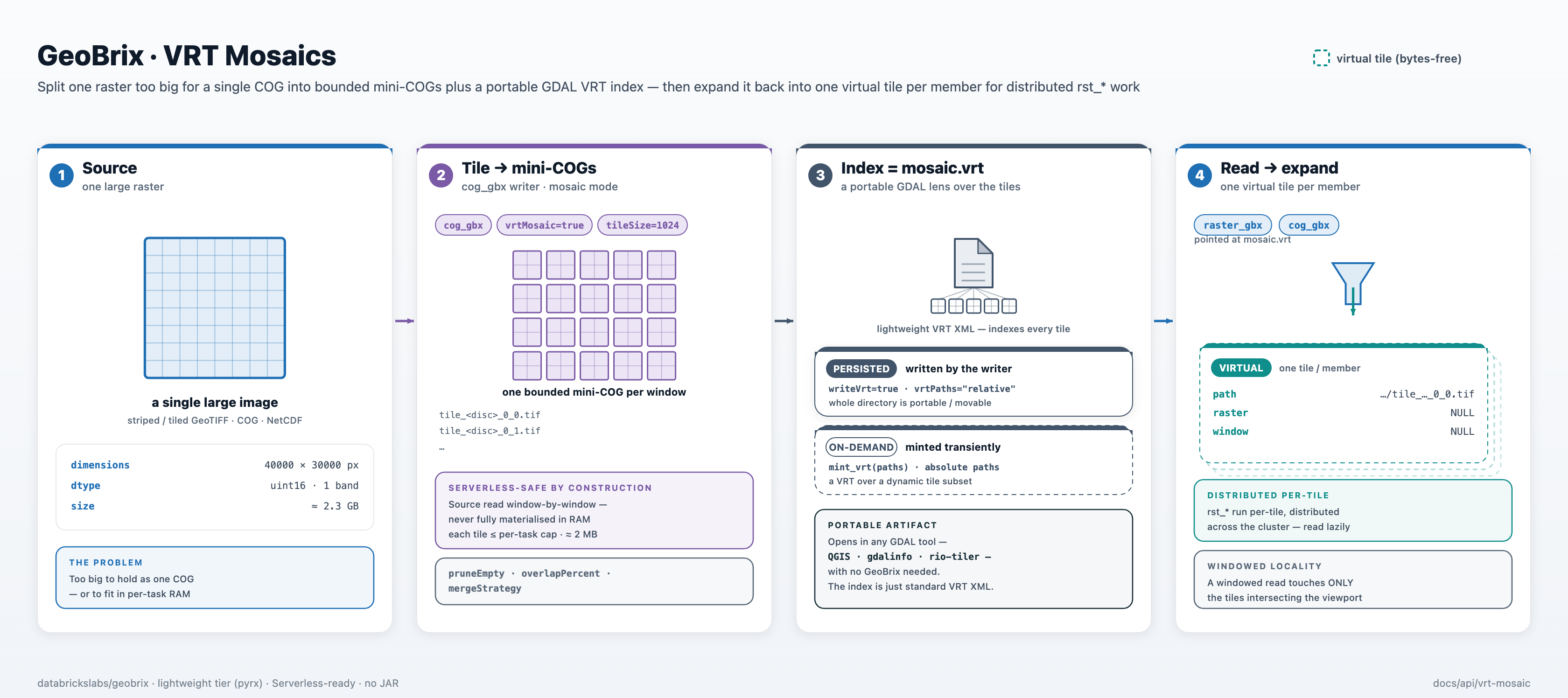
This complements the File Column table and Volume modes as a storage form for distributed raster processing:
| Form | What lives on disk | Best for |
|---|---|---|
| Single master COG | One large .tif per source | Windowed reads of one file at a time |
| VRT mosaic | Directory of mini-COGs + mosaic.vrt | Splitting sources that exceed per-task memory, portability across GDAL tools |
| FILE-column Delta table | FILE references in a Delta table | Governed, lifecycle-managed, long-term storage |
Prepare: write a VRT mosaic
Pass vrtMosaic=true to cog_gbx to enter mosaic mode. The writer reads each
source file window-by-window (one tile at a time — the source is never fully
materialised in RAM), writes one mini-COG per tile, and then builds mosaic.vrt
in the output directory. The tile grid defaults to gridSystem="none" (native
pixel tiling), so you normally set only vrtMosaic and, optionally, tileSize.
from databricks.labs.gbx.ds.register import register
register(spark)

# file_gbx gives one path-reference row per source file
sources = spark.read.format("file_gbx").load("/Volumes/catalog/schema/volume/raw/")

(
    sources
    .write.format("cog_gbx")
    .option("vrtMosaic", "true")   # activate mosaic mode
    .option("tileSize", "1024")    # tile edge in pixels (default 1024)
    .mode("overwrite")
    .save("/Volumes/catalog/schema/volume/mosaic/")
)
After the write, the output directory contains:
mosaic/
  tile_<discriminator>_0_0.tif   # mini-COG, row 0 col 0
  tile_<discriminator>_0_1.tif   # mini-COG, row 0 col 1
  ...
  mosaic.vrt                     # VRT index referencing all tiles
The <discriminator> is a stable, source-namespaced token
(up to 16 alphanum characters of the source basename + 8 hex characters of a
SHA-1 hash of the source path). Two sources in the same write never collide on
tile names, and a re-run produces the same names for the same sources
(cogSkipIfExists=true by default, so idempotent resumption is free).
Options
| Option | Default | Description |
|---|---|---|
vrtMosaic | — | Set "true" to activate VRT-mosaic mode. (Supplying gridSystem also activates it; one of the two must be present.) |
gridSystem | "none" | Tile grid. "none" (native pixel tiling, default), "quadbin" (cell-aligned to the quadbin grid, reprojected to EPSG:3857), "h3" (cell-aligned to the h3 grid, reprojected to EPSG:4326, hex-clipped), or "bng" (cell-aligned to the British National Grid, reprojected to EPSG:27700, square cells, Great Britain only). |
gridResolution | — | Grid resolution. Required when gridSystem="quadbin", gridSystem="h3", or gridSystem="bng"; invalid with gridSystem="none". Quadbin: range 0–20. H3: range 0–15. BNG: integer index ±1–±6 (1=100 km, 2=10 km, 3=1 km, 4=100 m, 5=10 m, 6=1 m) or string key (e.g. "1km", "100m"). |
tileSize | "1024" | Tile edge length in pixels. Tiles are square. The last row and column are clipped to the source boundary. |
overlapPercent | "0" | Tile-edge halo as a percentage of tileSize. A value of 5 expands each tile's read window by ceil(tileSize * 5 / 100) pixels on every side, clamped to the source bounds. Default 0 — non-overlapping grid. |
mergeStrategy | "none" | How overlapping tiles are blended: none (last-write wins), min, max, avg, first, or last. Relevant only when tiles from different sources overlap spatially. |
pruneEmpty | "true" | Skip tiles whose pixels are entirely NoData. Saves storage and reader work for sparse sources. |
writeVrt | "true" | Emit mosaic.vrt alongside the tiles. Set "false" if you only need the tiles and will build the index separately with mint_vrt. |
vrtPaths | "relative" | How tile paths are written inside the VRT. "relative" (default) — bare filenames, VRT is portable as long as tiles stay in the same directory. "absolute" — full paths, VRT works from any location. |
Mutually exclusive constraints:
driverMode=trueand mosaic mode cannot be combined — mosaic mode writes per-tile mini-COGs on executors;driverModeproduces a single driver-side COG. Use one or the other.tileSizeandoverlapPercentare only valid withgridSystem="none". DGGS-aligned options (gridMinResolution,gridMaxResolution,gridStepResolution) are reserved for future grid systems and are rejected forgridSystem="none".
Tile-encoding options (cogBlockSize, cogOverviewResampling, compress,
compressLevel, predictor, cogBigTiff, cogSkipIfExists) are passed
through to each mini-COG. See the COG Writer for the
full encoding option reference.
Quadbin (map-render) mosaic
When gridSystem="quadbin", the writer reprojects each source to EPSG:3857 and
writes one mini-COG per overlapping quadbin cell at the requested resolution.
Tiles are aligned to the quadbin grid, making the output directly compatible
with XYZ/quadkey map rendering pipelines and spatial join workflows that operate
on quadbin cell identifiers.
from databricks.labs.gbx.ds.register import register
from pyspark.sql.functions import col

register(spark)

# Write a quadbin mosaic: each source is reprojected to EPSG:3857 and split
# into one mini-COG per overlapping quadbin cell at the chosen resolution.
sources = spark.read.format("file_gbx").load("/Volumes/catalog/schema/volume/raw/")
(
    sources
    .write.format("cog_gbx")
    .option("gridSystem", "quadbin")   # cell-aligned to the quadbin grid
    .option("gridResolution", "7")     # quadbin resolution 0–20
    .mode("overwrite")
    .save("/Volumes/catalog/schema/volume/mosaic_qb/")
)

# Read back: one virtual tile per quadbin cell
df = spark.read.format("raster_gbx").load(
    "/Volumes/catalog/schema/volume/mosaic_qb/mosaic.vrt"
)

# tile.metadata carries the quadbin cell id and grid system tag
result = df.select(
    col("tile.path").alias("member"),
    col("tile.metadata")["cellid"].alias("cellid"),
    col("tile.metadata")["gridSystem"].alias("gridSystem"),
)
Cell tiles are named cell_<discriminator>_<cellid>.tif and the VRT index is
written as mosaic.vrt alongside them. The <discriminator> is the same stable
source-namespaced token used in native mode, so two sources in the same write
never collide.
When raster_gbx expands the VRT, each row's tile.metadata carries:
tile.metadata["cellid"]— the quadbin cell id (string)tile.metadata["gridSystem"]—"quadbin"
These fields are absent on native (gridSystem="none") tiles.
tileSize and overlapPercent are not valid with gridSystem="quadbin".
Set only gridSystem and gridResolution.
H3 (unification) mosaic
When gridSystem="h3", the writer reprojects each source to EPSG:4326 and
writes one mini-COG per overlapping h3 cell at the requested resolution. Each
cell's pixels are clipped to its hexagon boundary — pixels outside the hexagonal
footprint become NoData. This aligns the raster output to the h3 grid and makes
the cellid field a plain equi-join key for unifying with any other h3-indexed
dataset (gridded analytics, coverage tables, weather measurements, and similar).
from databricks.labs.gbx.ds.register import register
from pyspark.sql.functions import col

register(spark)

# Write an h3 mosaic: each source is reprojected to EPSG:4326, clipped to
# the hexagon boundary, and tagged with its h3 cell id (GBX_CELLID).
sources = spark.read.format("file_gbx").load("/Volumes/catalog/schema/volume/raw/")
(
    sources
    .write.format("cog_gbx")
    .option("gridSystem", "h3")      # cell-aligned to the h3 grid
    .option("gridResolution", "6")   # h3 resolution 0-15
    .mode("overwrite")
    .save("/Volumes/catalog/schema/volume/mosaic_h3/")
)

# Read back: one virtual tile per h3 cell
df = spark.read.format("raster_gbx").load(
    "/Volumes/catalog/schema/volume/mosaic_h3/mosaic.vrt"
)

# tile.metadata carries the h3 cell id and grid system tag
raster_cells = df.select(
    col("tile.path").alias("member"),
    col("tile.metadata")["cellid"].alias("cellid"),
    col("tile.metadata")["gridSystem"].alias("gridSystem"),
)

# Equi-join: any h3-indexed analytics table joins on cellid —
# the cellid is a plain string key, compatible with h3.str_to_int and similar.
analytics = spark.table("catalog.schema.h3_metrics")  # h3-indexed DataFrame
result = raster_cells.join(analytics, on="cellid", how="inner")
Cell tiles are named cell_<discriminator>_<h3index>.tif and the VRT index is
written as mosaic.vrt alongside them. The <discriminator> is the same stable
source-namespaced token used in native and quadbin modes, so two sources in the
same write never collide.
When raster_gbx expands the VRT, each row's tile.metadata carries:
tile.metadata["cellid"]— the h3 cell id (h3index string)tile.metadata["gridSystem"]—"h3"
The cellid value is the canonical h3index string — compatible with
h3.str_to_int / h3.int_to_str and with h3-indexed tables written by any
other workflow. Join the expanded mosaic rows to a tabular h3-indexed DataFrame
on cellid to unify raster pixel statistics with non-raster data sharing the
same grid.
tileSize and overlapPercent are not valid with gridSystem="h3".
Set only gridSystem and gridResolution.
BNG (British National Grid) mosaic
When gridSystem="bng", the writer reprojects each source to EPSG:27700 and
writes one mini-COG per overlapping BNG cell at the requested resolution. Tiles
are square and aligned to the British National Grid — the same cell boundaries
used by gbx_bng_* functions. This makes the output directly compatible with
BNG-indexed spatial join workflows and analytical pipelines that operate on BNG
cell identifiers.
BNG is valid over Great Britain only (EPSG:27700, approximately E 0–700 km, N 0–1300 km). A source outside this envelope produces no meaningful cells — its reprojected coverage is empty, so every candidate tile is all-nodata and pruned.
from databricks.labs.gbx.ds.register import register
from pyspark.sql.functions import col

register(spark)

# Write a BNG mosaic: each source is reprojected to EPSG:27700 and split into
# one mini-COG per overlapping BNG cell at the chosen resolution.
# BNG is valid over Great Britain only (EPSG:27700 extent).
sources = spark.read.format("file_gbx").load("/Volumes/catalog/schema/volume/raw/")
(
    sources
    .write.format("cog_gbx")
    .option("gridSystem", "bng")      # cell-aligned to the BNG grid (EPSG:27700)
    .option("gridResolution", "1km")  # BNG: integer index ±1..±6 or string key
    .mode("overwrite")
    .save("/Volumes/catalog/schema/volume/mosaic_bng/")
)

# Read back: one virtual tile per BNG cell
df = spark.read.format("raster_gbx").load(
    "/Volumes/catalog/schema/volume/mosaic_bng/mosaic.vrt"
)

# tile.metadata carries the BNG cell id and grid system tag
raster_cells = df.select(
    col("tile.path").alias("member"),
    col("tile.metadata")["cellid"].alias("cellid"),
    col("tile.metadata")["gridSystem"].alias("gridSystem"),
)

# Equi-join: any BNG-indexed analytics table joins on cellid —
# the cellid is a standard BNG string (e.g. "SU1234"), compatible with
# gbx_bng_* functions and any BNG-indexed dataset.
analytics = spark.table("catalog.schema.bng_metrics")  # BNG-indexed DataFrame
result = raster_cells.join(analytics, on="cellid", how="inner")
Cell tiles are named cell_<discriminator>_<cellid>.tif and the VRT index is
written as mosaic.vrt alongside them. The <discriminator> is the same stable
source-namespaced token used in native, quadbin, and h3 modes, so two sources in
the same write never collide.
When raster_gbx expands the VRT, each row's tile.metadata carries:
tile.metadata["cellid"]— the BNG cell id (string, e.g."SU1234")tile.metadata["gridSystem"]—"bng"
These fields are absent on native (gridSystem="none") tiles.
The cellid value is a standard BNG string compatible with gbx_bng_* functions.
Join the expanded mosaic rows to a tabular BNG-indexed DataFrame on cellid to
unify raster pixel statistics with non-raster data sharing the same grid.
tileSize and overlapPercent are not valid with gridSystem="bng".
Set only gridSystem and gridResolution.
Mint: on-demand VRT
mint_vrt builds a transient VRT over an arbitrary list of tile paths without
writing an index file alongside the tiles. The VRT is placed in a temporary
directory with absolute SourceFilename paths so rasterio can resolve each
member regardless of working directory.
from databricks.labs.gbx.ds._mosaic import mint_vrt

# Build a transient VRT over an explicit tile list
tile_paths = [
    "/Volumes/catalog/schema/vol/mosaic/tile_abc_0_0.tif",
    "/Volumes/catalog/schema/vol/mosaic/tile_abc_0_1.tif",
    "/Volumes/catalog/schema/vol/mosaic/tile_abc_1_0.tif",
]
vrt_path = mint_vrt(tile_paths)

# Open the VRT with rasterio for a windowed read across the mosaic
import rasterio
from rasterio.windows import Window

viewport = Window(col_off=400, row_off=200, width=600, height=400)
with rasterio.open(vrt_path) as vrt_ds:
    data = vrt_ds.read(window=viewport)
    # Only the tiles that intersect the viewport are read
Pass an explicit out path to write the VRT to a fixed location instead of a
temp directory. Choose the location by who needs to open the .vrt file, and
for how long — its member tiles are always referenced by absolute path, so
they must be reachable from wherever the VRT is opened:
# Driver-local, transient — a one-shot windowed read in this same process.
# /tmp is visible only to the driver and is gone when the driver restarts.
vrt_path = mint_vrt(tile_paths, out="/tmp/query_mosaic.vrt")

# Shared and durable — reopenable later, and readable by workers, another
# notebook, or an external GDAL tool (QGIS, gdalinfo, rio-tiler). The tiles it
# references must also live on the Volume so the absolute paths resolve there.
vrt_path = mint_vrt(tile_paths, out="/Volumes/catalog/schema/vol/mosaic/query.vrt")
A minted VRT is usable at a given place only if both the .vrt file and its
absolute member paths resolve there.
- No
out(temp dir) or a/tmppath — driver-local and ephemeral. This is the primary use ofmint_vrt: build a VRT over a dynamic tile subset, open it with rasterio in the same driver/notebook process for a windowed read, then discard it. It is invisible to workers and to later sessions, and you are responsible for deleting the temp file when you are done with it. - A
/Volumes/...path (FUSE) — shared across the driver, workers, and external clients, and it persists. Use it when the index must outlive the process or be read from somewhere else. Becausemint_vrtbakes absolute member paths, the tiles themselves must also be on the Volume.
If you instead want a portable, movable index co-located with its tiles — one
where you can copy or move the whole directory — prefer the writer's persisted
mosaic.vrt (writeVrt=true), which uses relative paths by default. A
minted VRT is the tool for a dynamic subset (pinned or ephemeral); the persisted
mosaic is the tool for the whole tile set.
mint_vrt is Connect-safe — pure Python + rasterio, no Spark session, no
_jvm, no osgeo. It can be called from a notebook driver cell or from
any Python process.
Parameters:
| Parameter | Required | Description |
|---|---|---|
tile_paths | Yes | Non-empty list of absolute paths to COG tiles. All tiles must share the same CRS, pixel size, band count, and dtype. |
out | No | Optional destination path for the VRT. When omitted, the VRT goes to a private temp directory (driver-local, transient). Put it on a Volume (/Volumes/...) if it must be reopened later or read from workers or other clients — see the reachability note above. |
Returns: absolute path (str) to the written VRT file.
Read: point a reader at the VRT
Point raster_gbx (or cog_gbx) at mosaic.vrt and the reader parses the
VRT XML, enumerates member paths, and emits one virtual tile row per member:
from databricks.labs.gbx.ds.register import register
from databricks.labs.gbx.pyrx.functions import rst_avg
from pyspark.sql.functions import col

register(spark)

# Load the VRT: one whole-file virtual tile per member mini-COG
df = spark.read.format("raster_gbx").load("/Volumes/catalog/schema/vol/mosaic/mosaic.vrt")

# Apply rst_* per tile — exactly as you would for a directory of flat files
result = df.select(
    col("tile.path").alias("member"),
    rst_avg(col("tile")).alias("avg"),
)
Each row is a whole-file virtual tile (raster=NULL, path set to the member
file path, window=NULL). All downstream rst_* functions operate on the tile
bytes read lazily from the member path on demand — no pixel data is loaded before
the operation actually needs it.
Directory vs. VRT load
When the load path points directly at mosaic.vrt the reader expands the
VRT into one row per member. When the load path points at the containing
directory the reader walks the directory for raster files and excludes
.vrt files — they are indexes, not raster members, and including them would
double-count the mosaic. Both patterns produce one row per tile, but the VRT
path is the canonical way to load a mosaic.
Spatial filtering
Pass clipPolygons to restrict the expansion to only the members that intersect
a given area of interest. Only the intersecting mini-COGs contribute rows; the
rest are skipped without being opened:
# Polygon in the CRS of the source raster
aoi_wkt = "POLYGON ((400000 4999000, 401000 4999000, 401000 5000000, 400000 5000000, 400000 4999000))"

df_clipped = (
    spark.read.format("raster_gbx")
    .option("clipPolygons", aoi_wkt)
    .option("clipCrs", "EPSG:32632")
    .load("/Volumes/catalog/schema/vol/mosaic/mosaic.vrt")
)
Serverless-safe by construction
Mosaic mode reads each tile window independently — the source is opened once
per executor task, and each tile is read as a bounded pixel array
(tileSize × tileSize × bands × itemsize). The source is never pulled fully
into memory. At the default tileSize=1024, a single-band uint16 tile is
approximately 2 MB — well within the Serverless per-task budget regardless of
how large the source raster is.
mint_vrt and _parse_vrt_members (the VRT parser inside the reader) are pure
Python — no GDAL Python bindings (osgeo), no native extension — so they work
identically on Serverless and on classic compute.
See Serverless & Memory for the full per-task memory model and guidance on routing large files.
What a VRT mosaic is good for
- Distributed processing of large rasters — a single source file too large
to process whole is split into bounded mini-COGs;
rst_*functions then run per-tile across the cluster. - Windowed locality — a windowed read via
mint_vrtorrasterio.open(vrt)touches only the mini-COGs whose spatial extent intersects the requested viewport. GDAL resolves the intersection from the VRT XML header without opening any tile that falls outside the window. - Portable GDAL artifact —
mosaic.vrtis a standard GDAL VRT file readable by QGIS, gdalinfo, rio-tiler, and any GDAL 2+ tool. WithvrtPaths="relative"(the default), the whole directory (tiles + VRT) can be copied or moved and the index stays valid. - Expandable to rows for distributed work — pointing any GeoBrix reader at
the VRT turns a static directory of tiles into a partitioned Spark DataFrame in
one line, feeding
rst_*pipelines without any manual enumeration.
Upcoming
In-notebook windowed rendering of a VRT mosaic is on the roadmap. Pyramid
options (gridMinResolution, gridMaxResolution, gridStepResolution) are
accepted by the parser but raise a clear error until their grid-system support
lands.
See also
- Large Rasters — COG preparation, the memory model, and when to split a large source into a mosaic
- Virtual Tiles — how VRT expansion fits into the virtual/materialized tile lifecycle
- COG Writer (
cog_gbx) — full option reference for the COG preparation writer - COG Reader (
cog_gbx) — windowed, bbox-clipped reads from prepared COGs - Serverless & Memory — Serverless per-task memory model and safe write patterns