Virtual Tiles

Reading a multi-gigabyte raster the naïve way pulls the whole image into memory — and fanning it into pieces multiplies that cost until an executor runs out of memory. GeoBrix avoids this with virtual tiles: each row of the DataFrame carries a reference to a window of a raster — a path plus a pixel window — instead of the pixels themselves. Pixels are read lazily, one window at a time, only when an operation actually needs them.

This page explains the virtual-tile model, why it dissolves the ingest-memory problem, and how tiles move between virtual (bytes-free) and materialized (bytes-in-hand) states across the read → operate → write lifecycle.

What a virtual tile is

Every GeoBrix raster tile is one typed struct — the v2 tile struct — shared by both execution tiers:

struct<
  cellid: bigint,                       -- grid cell id (nullable)
  raster: binary,                       -- the raster payload (NULL when virtual)
  path: string,                         -- source path (set when virtual)
  window: struct<col_off,row_off,width,height>,  -- the pixel window
  clip_polygon: binary,                 -- optional clip geometry (WKB)
  clip_crs: string,                     -- CRS for clip_polygon
  crs: string,                          -- working/target CRS
  metadata: map<string,string>,         -- driver, extension, format keys
  path_mode: string                     -- storage mode: null, 'external', or 'managed'
>

A tile is virtual when raster is NULL and path + window are set — it is a bytes-free reference to a window of a raster on durable storage. A tile is materialized when raster carries the encoded bytes. The struct is identical either way, so a DataFrame can hold a mix, and a tile can move between the two states without changing shape. See Tile Structure for a field-by-field reference to this struct.

Reference vs. instruction

The window / clip_polygon / clip_crs / crs fields mean different things depending on the tile's state, and this is the key to reasoning about them:

• On a materialized tile they are provenance — a record of what has already been applied to produce the bytes in raster.
• On a virtual tile they are instructions — pending operations that are applied when the tile is read (staged from path, the window extracted, the clip and CRS applied), producing the pixels on demand.

Why it matters

Carrying references instead of pixels is what makes large-raster ingest scale:

• Bytes-free rows. A virtual tile row is roughly 100 bytes (a path and a four-integer window). The materialized bytes it stands in for are 148–527 KB per tile — so virtual rows are on the order of 1,400–5,000× smaller. At ingest you hold N tiny descriptor rows instead of hundreds of MiB of encoded tiles, and the accumulation that causes Serverless out-of-memory failures simply does not happen.
• Windowed, parallel reads. Readers fan a source out across the cluster — one window per tile, one tile per task — and each window is a small ranged read against a Cloud-Optimized GeoTIFF. No executor ever holds the whole image, and there is no driver-side collect.
• Lazy composition. Deferrable operations chain on virtual tiles without ever touching pixels — the DataFrame keeps carrying references until an operation genuinely needs the data.

This is the cloud-native raster model — don't move pixels; read windows on demand — expressed as a Spark DataFrame.

The lifecycle

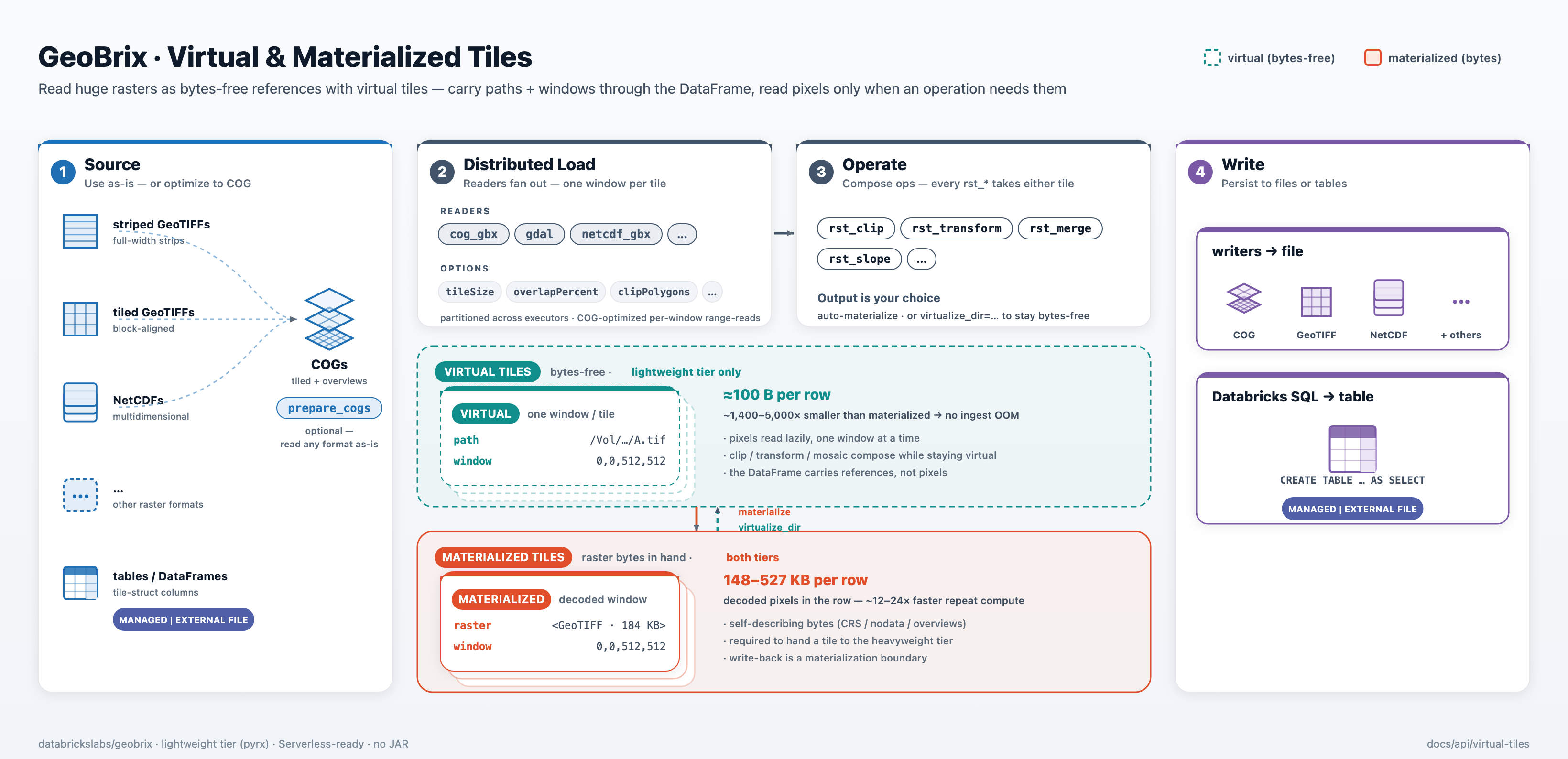
The diagram above traces the four stages:

1. Source. Striped GeoTIFFs, tiled GeoTIFFs, COGs, NetCDFs, and tabular tile-struct columns are all usable as-is. File formats can optionally be standardized into COGs first with prepare_cogs, which makes windowed reads cheap (a striped source can inflate a single window ~570× versus a clean tiled block). Optimization is a choice, not a gate.
2. Distributed load. A reader (cog_gbx, gdal, netcdf_gbx, …) partitions the source across executors and emits tile rows — the lightweight raster readers (raster_gbx, gtiff_gbx, cog_gbx) emit virtual tiles by default; pass .option("virtualTiles", "false") to get materialized bytes instead. Selection options (tileSize, overlapPercent, clipPolygons, …) shape the windowing.
3. Operate. Any rst_* function accepts either a virtual or a materialized tile. The output shape is your choice — see below.
4. Write. Persist to files (COG, GeoTIFF, NetCDF, …) with a writer, or save a tile DataFrame to a Databricks SQL table.

Virtual Tiles + FILE

FILE is a Databricks data type that provides governed access to files on compute without a FUSE mount. GeoBrix detects FILE availability and uses it when present. If FILE is not available, virtual tiles work via the FUSE path unchanged.

When FILE is available (Databricks Runtime 19 dedicated clusters), GeoBrix:

• Stamps each virtual tile row with a path_mode field: "external" or "managed" (see Tile Structure).
• Opens the file via fref.open() (byte-range stream) rather than through the FUSE mount.
• Falls back gracefully to the FUSE path if the FILE feature-detect fails.

Key point: A FileRef is minted and consumed within each tile operation, then discarded. It is never stored as a DataFrame column and does not affect the tile struct's public shape.

Read performance with FILE

The decisive factor for virtual-tile read performance is open amortization — opening a source raster once and reading many windows from that handle, rather than once per tile. Under the grouped executor pattern (per-partition LRU of open stream handles), byte-range stream reads are 10–290× faster than FUSE for windowed COG reads. Without amortization (per-tile-open), the per-open cost of a stream scales with file size and can become prohibitive. See Virtual tile read performance for the full benchmark data, handling rules, and write-layout guidance.

Supported environments

• Databricks Runtime 19 dedicated clusters (single-user, with fileReferenceCreationMode=MANAGED in cluster config): FILE engages where the runtime feature-detect succeeds. Where it does not, tiles use FUSE automatically.
• Databricks Runtime 19 on Serverless: coming soon.
• Local development, CI, Serverless Compute (today), DBR 17/18: virtual tiles use the traditional FUSE + rasterio path — correct and unchanged.

Reader selection surface

The lightweight readers expose the windowing surface as read options:

• virtualTiles — emit bytes-free virtual tiles (true, the default) or materialized tiles (false).
• tileSize — regular tiling grid; overlapPercent — overlap between adjacent tiles so per-tile operations don't clip features at the edges.
• clipPolygons / clipCrs — emit only the tile(s) intersecting each polygon; windows — explicit pixel windows.

See the cog_gbx reader and the Readers overview for the full option reference — this page does not duplicate them.

Many-file directories

When a directory contains thousands of small tiles, loading it with .load(dir) incurs planning overhead even with virtual tiles: the reader still walks the directory and opens each header to compute window dimensions. Measured on a 10,002-file corpus, a pre-computed manifest drops plan time from 1.357 s to 0.037 s — about 37× faster. Use the manifest or tilesTable reader option to supply pre-computed tile paths and windows, reducing planning to a single file or table read regardless of tile count. See Raster Reader performance and Benchmarking → Reader plan-time listing.

Operating on tiles: your choice of output

Every lightweight tile-returning rst_* function takes three optional force-output parameters:

• virtualize_dir — write the produced tile to a durable path and hand back a virtual row (bytes-free), so a chain stays light after a pixel-producing op.
• virtualize_prefix — an optional filename prefix to deconflict outputs.
• materialize — force raster bytes into the row.

The default is automatic: reference/passthrough operations stay virtual, and pixel-producing operations materialize — but you can always ask for the other. For the full rule (which operations are free on virtual tiles and which materialize), see the Virtual↔materialized advice on the Execution Tiers page.

Instructions that stay virtual

A few cheap, common operations record an instruction on a virtual tile instead of reading pixels — the tile stays bytes-free and the instruction is applied on the next read (alongside the window and any clip/reproject):

• rst_initnodata — set the NoData value
• rst_setsrid — relabel the CRS (assign an EPSG code; not a reproject)
• rst_band — select a band

They accumulate: chain them on a virtual tile and all apply together when the tile is finally read (e.g. at tessellation). Pass materialize=True (or virtualize_dir) to apply them immediately and produce bytes.

Tiers: light tiles vs. heavy tiles

The lightweight tier is for light (virtual) raster tiles; the heavyweight tier is for heavy (binary) raster tiles.

• The lightweight tier (pyrx) generates and operates on virtual tiles, and materializes them on demand. Virtual tiles are a lightweight-tier capability.
• The heavyweight tier (rasterx) accepts both v1 and v2 materialized tiles as input and always emits the v2 tile struct. It operates only on materialized tiles: a virtual tile passed to a heavyweight function raises a clear error telling you to materialize it first (call the lightweight function with materialize=True, or write it out and read it back). Writing is itself a materialization boundary.

See also

• Large Rasters — preparing COGs at scale (prepare_cogs, cog_gbx driverMode) and the format/memory details behind windowed reads.
• VRT & Mosaics — a .vrt index over mini-COG tiles expands into one virtual tile row per member; rst_* functions run per-tile unchanged.
• Execution Tiers — the full virtual↔materialized taxonomy and the light→heavy bridge.
• COG reader (cog_gbx) and Readers overview — the windowed-read option reference.
• Writers overview — persisting tiles to files.