Multi-Layer Compositor
A single GeoBrix analysis often produces several result layers at once — vector zone boundaries, a raster DEM, discrete H3 grid cells, and a pre-tiled PMTiles archive. plot_static and plot_interactive accept a list of layers and composite them in order, so one function call produces one map.
When the total GeoJSON + PNG payload fits within the embed budget (small by default in a notebook — see the ladder below), plot_interactive embeds everything inline in the HTML string — no tile server, no separate request. When it doesn't fit, the embed-size ladder picks the right path automatically. The runnable example below composites two vector layers; raster- and grid-layer usage is shown in the Vector and Raster references.
The compositor requires geobrix[vizx]. Install with:
pip install "geobrix[vizx]"
Layer types
Each constructor returns a Layer object. Pass a list of them to plot_static or plot_interactive.
| Constructor | Typical input | Notes |
|---|---|---|
vector_layer(data) | geopandas.GeoDataFrame, Spark DataFrame, WKT/WKB | Accepts any geometry encoding. |
raster_layer(data) | COG/raster file path, numpy.ndarray, or tile struct | Path → rasterio; ndarray → unit-square corners. |
grid_layer(data, grid_system=) | DataFrame of H3 / BNG / Quadbin cell ids | Requires grid_system='h3', 'bng', 'quadbin', or 'custom'. |
pmtiles_layer(data) | .pmtiles bytes, local path, or https:// URL | URL mode streams from the remote server with zero embed cost. |
from databricks.labs.gbx.vizx import (
    vector_layer,
    raster_layer,
    grid_layer,
    pmtiles_layer,
    plot_static,
    plot_interactive,
)
Each constructor exposes a label= argument used in audit output and map legends.
Data-driven color scale
vector_layer and grid_layer color each feature/cell by a column= through a matplotlib cmap=. The scale= argument controls how values map onto the colormap:
scale | Mapping | Use when |
|---|---|---|
"linear" (default) | Ramp position = (value − min) / (max − min) | Values are roughly uniform across their range. |
"quantile" | Ramp position = the value's percentile rank | Values are skewed — a dense low range with a long tail. |
Linear normalization crushes a skewed distribution into one end of the ramp: if most cells hold a small value with a few large outliers (e.g. roof counts of 1–25 in a 1–128 range), nearly every cell renders as the same pale color. "quantile" spreads the dense range across the full ramp so those cells stay distinguishable; the legend gains a median tick to keep the (non-linear) mapping honest.
from databricks.labs.gbx.vizx import grid_layer, plot_interactive

# H3 roof-density heatmap — quantile so the crowded low range stays readable
plot_interactive([
    grid_layer(
        cells_df, grid_system="h3", cellid_col="h3_cell",
        column="n_roofs", cmap="YlOrRd", scale="quantile", label="roofs / cell",
    )
])
The embed-size ladder
When total payload grows beyond the embed budget, plot_interactive walks through a four-rung ladder to find the right delivery strategy:
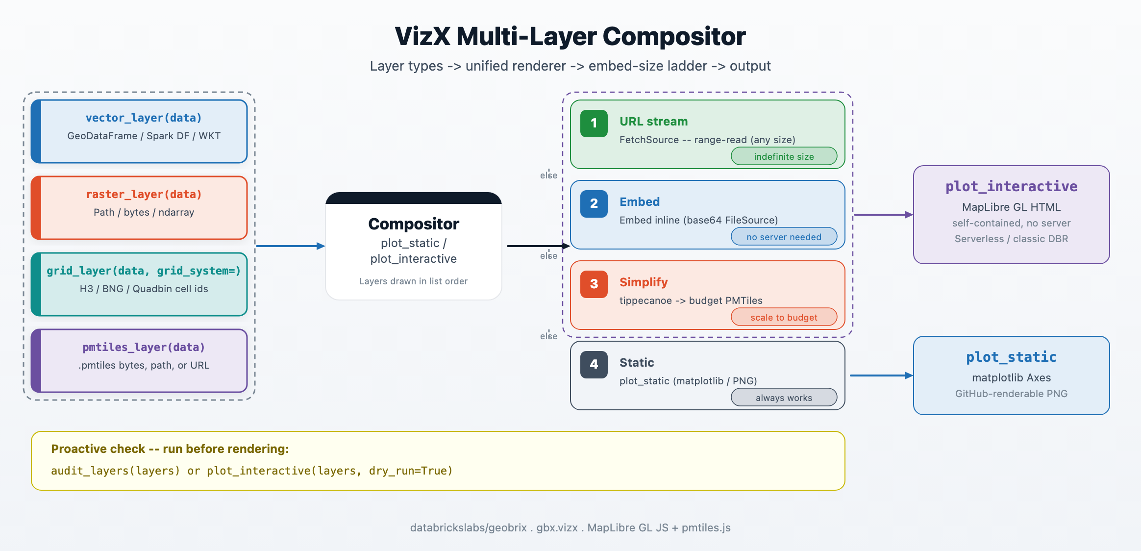
| Rung | Condition | Delivery |
|---|---|---|
| 1 — URL | pmtiles_layer carries an https:// URL | FetchSource range-reads on demand; zero embed cost. |
| 2 — embed | Total HTML size ≤ max_embed_mb (default ~3 MB, ~6 MB with the raised cell cap) | Base64 FileSource in-browser; no server, no network at render time. |
| 3 — simplify | Over budget, simplify_tiles_spec= provided | Runs tippecanoe to produce a budget-sized PMTiles archive, then re-embeds. |
| 4 — static | Over budget, no simplify path | Falls back to plot_static; GitHub-renderable PNG. |
The max_embed_mb threshold applies to the assembled HTML byte length, not to individual layer sizes. In a Databricks notebook the practical ceiling is lower still: cell output is capped (~10 MB default, 20 MB max — vizx raises it automatically), and displayHTML inflates the payload ~2–3×, so an archive over ~4–5 MB takes rung 3 or 4 rather than embedding.
Multi-layer static composite
plot_static draws each layer in order on a single matplotlib.Axes and returns it. Layers are reprojected to Web Mercator (EPSG:3857) so they align with one another and with any basemap. Pass basemap=False for a deterministic, offline-safe render.
import matplotlib.pyplot as plt

from databricks.labs.gbx.vizx import plot_static, vector_layer

plt.close("all")

gdf_poly = _small_polygon_gdf()
gdf_pts = _small_point_gdf()

# Layer order: polygon footprint on the bottom, point sites on top.
layers = [
    vector_layer(gdf_poly, color="#3388ff", opacity=0.5, label="zones"),
    vector_layer(gdf_pts, color="#e04e2a", label="sites"),
]
ax = plot_static(layers, basemap=False)

assert ax is not None, "plot_static should return an Axes"
children = ax.get_children()
assert len(children) >= 2, f"Expected >=2 artists on the axes, got {len(children)}"
plt.close("all")
The static path renders every listed layer type except pmtiles_layer (which emits a warning and produces no output — use plot_interactive for PMTiles, or let the budget ladder decode them automatically on the fallback path).
Multi-layer interactive map
plot_interactive converts each layer to MapLibre GL sources, assembles one self-contained HTML string, and either embeds it inline or streams it from a URL depending on the embed-size ladder above. Use dry_run=True to inspect the size audit without rendering.
from databricks.labs.gbx.vizx import plot_interactive, vector_layer

gdf_pts = _small_point_gdf()
gdf_poly = _small_polygon_gdf()

layers = [
    vector_layer(gdf_poly, color="#e04e2a", opacity=0.5, label="zones"),
    vector_layer(gdf_pts, color="#1f6fb5", label="sites"),
]
# dry_run=True returns the audit dict without calling displayHTML.
# This works both inside and outside a notebook environment.
result = plot_interactive(layers, basemap="carto-positron", dry_run=True)

assert isinstance(result, dict), "Expected audit dict from dry_run=True"
assert result["fits"] is True, f"Small layers should fit: {result}"
assert result["verdict"] == "embed", f"Expected 'embed', got {result['verdict']!r}"
assert len(result["layers"]) == 2, f"Expected 2 layers, got {len(result['layers'])}"
assert result["layers"][0]["label"] == "zones"
assert result["layers"][1]["label"] == "sites"
In a Databricks notebook, omit dry_run=True and plot_interactive calls displayHTML automatically. Outside a notebook (plain Python, tests), it returns the HTML string.
Proactive audit: never a surprise
Call audit_layers before rendering to see exactly how much budget each layer consumes and which rung the compositor will select.
from databricks.labs.gbx.vizx import audit_layers, vector_layer

gdf = _small_polygon_gdf()
layers = [vector_layer(gdf, label="zones")]
result = audit_layers(layers, max_embed_mb=64)

assert "fits" in result, "audit dict must have 'fits'"
assert "verdict" in result, "audit dict must have 'verdict'"
assert "total_embed_bytes" in result, "audit dict must have 'total_embed_bytes'"
assert result["fits"] is True, f"Small GeoDataFrame should fit in 64 MB: {result}"
assert result["verdict"] == "embed", (
    f"Expected verdict='embed', got {result['verdict']!r}"
)
assert result["total_embed_bytes"] > 0
The returned dict has the following keys:
| Key | Type | Description |
|---|---|---|
fits | bool | True when total HTML size is within the budget. |
verdict | str | "embed", "url", "simplify", or "static". |
total_embed_bytes | int | Actual assembled-HTML byte length. |
max_embed_bytes | int | Budget in bytes (max_embed_mb * 1_048_576). |
layers | list[dict] | Per-layer breakdown: label, kind, embed_bytes, max_tile_bytes. |
plot_interactive(layers, dry_run=True) is an equivalent one-liner that also prints the audit line without rendering.
Ephemeral vs durable simplification
When the embed budget is tight, simplify_tiles_from_source lets you pre-tile data into a compact PMTiles archive with tippecanoe. The result can be held in memory (ephemeral) or written to a path (durable).
Ephemeral — bytes returned directly, held in driver memory:
if shutil.which("tippecanoe") is None:
    # tippecanoe absent — skip gracefully in non-vizx environments.
    return None

from databricks.labs.gbx.vizx import simplify_tiles_from_source

gdf = _small_polygon_gdf()
result = simplify_tiles_from_source(gdf, spec={"max_z": 6, "min_z": 0})

assert isinstance(result, (bytes, bytearray)), "Expected bytes"
assert len(result) > 0, "PMTiles bytes should be non-empty"
assert result[:7] == b"PMTiles", "Should start with PMTiles magic bytes"
Durable — written to a file path, reusable across sessions:
if shutil.which("tippecanoe") is None:
    return None

from databricks.labs.gbx.vizx import simplify_tiles_from_source

gdf = _small_polygon_gdf()
out = os.path.join(tmp_path, "overview.pmtiles")
result = simplify_tiles_from_source(gdf, spec={"max_z": 5}, out_path=out)

assert result == out, f"Return value should be out_path, got {result!r}"
assert os.path.exists(out), f"File should exist at {out}"
with open(out, "rb") as f:
    header = f.read(7)
assert header == b"PMTiles", "File should be a valid PMTiles archive"
If you already have a PMTiles archive and only need an overview embed (for example, cutting a detailed 0–14 archive down so it fits an interactive cell), you don't need to re-tile from source. Pass the archive to plot_pmtiles(archive, interactive_fit="downzoom") — the interactive embedder drops the highest (densest) zoom levels until the rendered archive fits the embed budget. This reduction is binary-free (no tippecanoe) and works for both raster and vector tiles, since it rebuilds a smaller archive from the tiles already present.
simplify_tiles_from_source requires the tippecanoe binary (the interactive_fit="downzoom" archive reduction above does not).
pip install "geobrix[vizx]" installs the tippecanoe Python wheel (manylinux), so Databricks clusters and Serverless are covered automatically — no extra step needed.
On macOS (especially Apple Silicon) the manylinux wheel may be unavailable or unreliable; use brew install tippecanoe as a fallback. The rest of VizX (plotting, compositing, audit) works without tippecanoe.
Once you have a durable archive, pass it to pmtiles_layer and embed it or stream it from a Volume URL:
from databricks.labs.gbx.vizx import pmtiles_layer, plot_interactive

# Embed a pre-tiled overview archive
layers = [pmtiles_layer("overview.pmtiles", label="overview")]
plot_interactive(layers)

# Stream from a Volume URL (zero embed cost, any size)
layers = [pmtiles_layer(
    "https://<workspace>.azuredatabricks.net/api/2.0/fs/files/Volumes/.../overview.pmtiles",
    label="overview",
)]
plot_interactive(layers)
Scale guidance
The default embed budget is intentionally small — a few MB — because a Databricks notebook caps cell output (~10 MB, 20 MB max) and displayHTML inflates the payload ~2–3×, capping the inline archive at ~4–5 MB. Modest vector layers embed comfortably; when your data is larger:
- Pre-tile with
simplify_tiles_from_sourceto generate a compact overview archive, then embed or stream it. - Stage the archive on a Volumes URL and use
pmtiles_layer("https://...")— URL mode has zero embed cost regardless of archive size. - For very large datasets requiring distributed tile generation, the Helios notebooks show how to produce multi-shard PMTiles archives with
gbx_pmtiles_aggand serve them directly.
Dynamic zoom cut-over (live kernel). plot_interactive_dynamic(layers, simplify_tiles_spec=…) embeds a low-zoom overview of the archive inline and streams higher-zoom detail on pan/zoom (with optional neighbour prefetch). This avoids serving the full archive at once, so it stretches the usable embed budget further. It requires a live kernel — it is an ipywidget and does not render in a committed .ipynb on GitHub or in the docs site; the static composite covers that surface.
Beyond the embed budget — Databricks App tile server. When a single archive is too large even for the dynamic cut-over, or when you need indefinite interactivity for end users outside a notebook, the long-term path is a Databricks App that acts as a tile server backed by your PMTiles archive on Volumes. This is a planned capability; for now, URL-mode streaming (pmtiles_layer("https://...")) and multi-shard archives via gbx_pmtiles_agg cover most production cases.
The static fallback (plot_static) is always available as a last resort. It produces a GitHub-renderable PNG that bakes the basemap in at execution time via contextily — no network needed at render time, and the output displays correctly on GitHub and in docs.
Next steps
- VizX Function Reference — raster plotters, vector adapters,
plot_cog - PMTiles functions — building and inspecting PMTiles archives
- Helios notebooks — end-to-end: vector + raster + PMTiles in one notebook