Kepler visualizations

You can use the %%mosaic_kepler magic function to visualise data using Kepler.gl.

The mosaic_kepler magic function accepts four parameters:

1. dataset: Can be a Spark dataset or a string representing a table/view name

2. column_name: The column that needs to be plotted, can be either a geometry column (WKT, WKB or Mosaic internal format) or a column containing a spatial grid index ID

3. feature_type: The type of data to be plotted. Valid values are geometry (if SRID=4326), geometry(<SRID>) (where <SRID> is the SRID used by the geometry column), geometry(bng), geometry(osgb36), bng and h3

4. limit: The maximum number of objects to plot. The default limit is 1000

Usage:

%%mosaic_kepler
dataset column_name feature_type [limit]

This magic function is only available in python. It can be used from notebooks with other default languages by storing the intermediate result in a temporary view, and then adding a python cell that uses the mosaic_kepler with the temporary view created from another language.

Examples

%pip install databricks-mosaic --quiet

Python interpreter will be restarted. Python interpreter will be restarted.

from pyspark.sql.functions import *
import mosaic as mos
mos.enable_mosaic(spark, dbutils)

Download example shapes

import requests

req = requests.get('https://data.cityofnewyork.us/api/geospatial/d3c5-ddgc?method=export&format=GeoJSON')
with open('/dbfs/tmp/nyc_taxi_zones.geojson', 'wb') as f:
  f.write(req.content)

neighbourhoods = (
  spark.read
    .option("multiline", "true")
    .format("json")
    .load("dbfs:/tmp/nyc_taxi_zones.geojson")

    # Extract geoJSON values for shapes
    .select("type", explode(col("features")).alias("feature"))
    .select("type", col("feature.properties").alias("properties"), to_json(col("feature.geometry")).alias("geom_json"))

    # Mosaic internal representation
    .withColumn("geom_internal", mos.st_geomfromgeojson("geom_json"))

    # WKT representation
    .withColumn("geom_wkt", mos.st_aswkt(col("geom_internal")))

    # WKB representation
    .withColumn("geom_wkb", mos.st_aswkb(col("geom_internal")))

   # Limit to only 1 shape
   .limit(1)
)

neighbourhoods.show()

+-----------------+--------------------+--------------------+--------------------+--------------------+--------------------+ type| properties| geom_json| geom_internal| geom_wkt| geom_wkb| +-----------------+--------------------+--------------------+--------------------+--------------------+--------------------+ FeatureCollection|{EWR, 1, 1, 0.000...|{"coordinates":[[...|{6, 4326, [[[-74....|MULTIPOLYGON (((-...|[01 06 00 00 00 0...| +-----------------+--------------------+--------------------+--------------------+--------------------+--------------------+

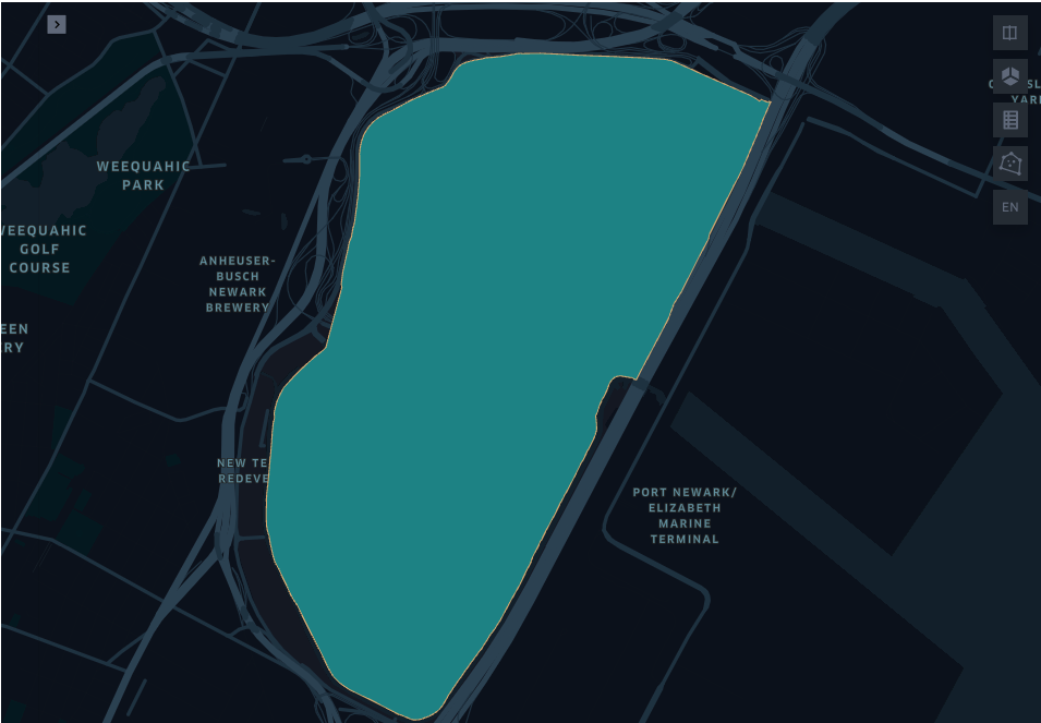
Plot geometries from Spark dataset

Internal geometry type

%%mosaic_kepler
neighbourhoods "geom_internal" "geometry"

User Guide: https://docs.kepler.gl/docs/keplergl-jupyter

WKT geometry type

%%mosaic_kepler
neighbourhoods "geom_wkt" "geometry"

User Guide: https://docs.kepler.gl/docs/keplergl-jupyter

WKB geometry type

%%mosaic_kepler
neighbourhoods "geom_wkb" "geometry"

User Guide: https://docs.kepler.gl/docs/keplergl-jupyter

Plot geometries from table/view

neighbourhoods.createOrReplaceTempView("temp_view_neighbourhoods")

%%mosaic_kepler
"temp_view_neighbourhoods" "geom_wkt" "geometry"

User Guide: https://docs.kepler.gl/docs/keplergl-jupyter

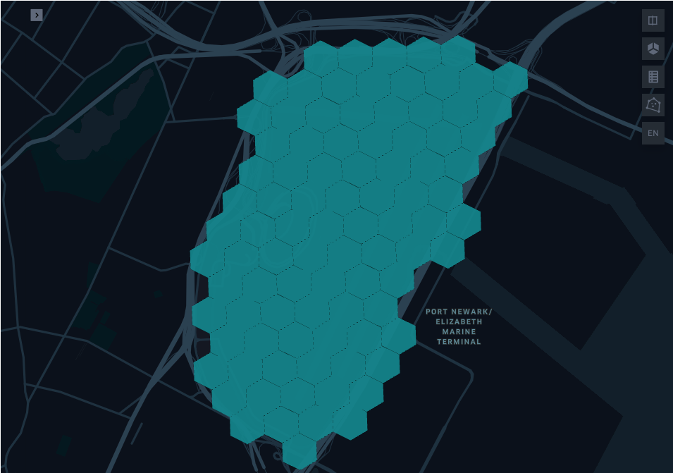
Plot H3 indexes

neighbourhood_chips = (neighbourhoods
                       .limit(1)
                       .select(mos.grid_tessellateexplode("geom_internal", lit(9)))
                       .select("index.*")
                    )

neighbourhood_chips.show()

+-------+------------------+--------------------+ is_core| index_id| wkb| +-------+------------------+--------------------+ true|617733150781997055|[01 03 00 00 00 0...| true|617733150856445951|[01 03 00 00 00 0...| true|617733150856970239|[01 03 00 00 00 0...| true|617733150784094207|[01 03 00 00 00 0...| true|617733150843600895|[01 03 00 00 00 0...| true|617733150843863039|[01 03 00 00 00 0...| true|617733150844125183|[01 03 00 00 00 0...| true|617733150784880639|[01 03 00 00 00 0...| true|617733150844387327|[01 03 00 00 00 0...| true|617733150844649471|[01 03 00 00 00 0...| true|617733150785404927|[01 03 00 00 00 0...| true|617733150844911615|[01 03 00 00 00 0...| true|617733150785667071|[01 03 00 00 00 0...| true|617733150845173759|[01 03 00 00 00 0...| true|617733150785929215|[01 03 00 00 00 0...| true|617733150786453503|[01 03 00 00 00 0...| true|617733150846222335|[01 03 00 00 00 0...| true|617733150847270911|[01 03 00 00 00 0...| true|617733150847795199|[01 03 00 00 00 0...| true|617733150848057343|[01 03 00 00 00 0...| +-------+------------------+--------------------+ only showing top 20 rows

%%mosaic_kepler
neighbourhood_chips "index_id" "h3"

User Guide: https://docs.kepler.gl/docs/keplergl-jupyter

Plot H3 chips

%%mosaic_kepler
neighbourhood_chips "wkb" "geometry"

User Guide: https://docs.kepler.gl/docs/keplergl-jupyter